<?xml version="1.0" encoding="utf-8"?><feed xmlns="http://www.w3.org/2005/Atom" ><generator uri="https://jekyllrb.com/" version="3.10.0">Jekyll</generator><link href="/feed.xml" rel="self" type="application/atom+xml" /><link href="/" rel="alternate" type="text/html" /><updated>2026-10-01T03:00:32+00:00</updated><id>/feed.xml</id><title type="html">Benjamin Clarke</title><subtitle>Data Scientist committed to continual learning and discovery</subtitle><entry><title type="html">Getting to know Graph ML</title><link href="/blog/intro_graph_ml" rel="alternate" type="text/html" title="Getting to know Graph ML" /><published>2026-09-30T00:00:00+00:00</published><updated>2026-09-30T00:00:00+00:00</updated><id>/blog/intro-graph-ml</id><content type="html" xml:base="/blog/intro_graph_ml"><![CDATA[<p>In my previous post, I mentioned that I’ve been exploring the use of graph methods in modeling and deep learning, some for work and some for my own hobby projects.<br />
Because I spent much of September traveling and resting before starting a new grad program, I haven’t had a lot of time recently for diving more into this topic, but I wanted to put together a short post summarizing the things I’ve learned so far to lay the groundwork for future posts on graph models.</p>

<h2 id="technical-background">Technical background</h2>

<p>I’ve been fascinated by graph theory ever since taking a combinatorics class back in college, and I wish I had more time that I could use to study the topic more deeply. Graph theory has a storied history stretching back to <a href="https://en.wikipedia.org/wiki/Seven_Bridges_of_K%C3%B6nigsberg">Euler</a> in the eighteenth century, and the uses cases abound from route planning to recommendation systems.  I won’t go into the fundamentals of graph structures here, but you can find a number of good tutorials online; <a href="https://huggingface.co/blog/intro-graphml">this</a> walkthrough from huggingface would be a good place to start. <br />
Prior to the big data revolution, graph models primarily focused on extracting features and calculating metrics for gaining insights. Some examples of node-level features would be centrality, degree, and the clustering coefficient; edge-level features included shortest distance, common neighbors, and Katz index (number of possible walks between nodes); examples of graph-level features would be total subgraphs and kernel methods for similarity scores.<br />
The sorts of features could be fed into classical algorithms that aimed to answer questions around centrality, shortest paths, types of subgraphs, etc. Neo4j has a good intro <a href="https://neo4j.com/blog/graph-data-science/graph-algorithms/">guide</a> to these sorts of algorithms. <a href="https://neo4j.com/docs/graph-data-science/current/getting-started/">Neo4j</a> is a popular system for storage, exploration, and modeling of graphs; I haven’t played around with it too much, but the visualizations definitely look pretty.</p>

<h2 id="the-increasing-relevance-of-graph-models">The increasing relevance of graph models</h2>

<p>Despite being studied for so long, graph models have only continued to grow in importance. Increasing data collection from social networking companies, streaming media services, and many others often deal with data where relationships between customers or products contain vital information for the sorts of questions being asked.<br />
Use cases for graph models fall into both supervised and unsupervised categories:</p>

<p><strong>Supervised tasks:</strong></p>

<ul>
  <li>Node property prediction - node classifcation, node regression</li>
  <li>Link prediction - whether or not a link should exist, and potentially what type</li>
  <li>Graph property prediction - structure of a graph, types of subgraphs</li>
</ul>

<p><strong>Unsupervised tasks:</strong></p>

<ul>
  <li>Representation learning - generate features based on graph structure for another model</li>
  <li>Clustering/Community Detection - groups of nodes that go together</li>
  <li>Similarity - find pairs of nodes that go together; use cases such as recommendation, entity resolution</li>
  <li>Centrality &amp; Pathfinding - find important entities in the graph, evaluate efficient paths and trees</li>
</ul>

<p>Additionally, graphs can get huge. The combinatorial explosion of connections means that even for graphs where nodes only have a few connections on average, the size of the data structure can increase exponentially. <br />
Given this increase in size as well as relevance for graph data, many of these classical methods of studying graphs, as well as the standard table data structures in which databases often store them, can struggle to keep up.</p>

<p>With a prime source of big data (the graphs) and a plethora of use cases, the idea naturally arises to apply machine learning to the problem.</p>

<h2 id="incorporation-into-machine-learning">Incorporation into Machine learning</h2>

<p>Many of the types of deep learning architectures don’t transfer perfectly into the domain of graph structures, because they are unable to capture the information contained in the relationships between nodes communicated by links. The standard deep learning models have a tough time capturing the information contained within multiple connections, as well as aspects such as path directions. CNNs pull information from connections between a data point’s immediate neighbors, but they are limited in their reach. The Transformer comes closer as one could potentially envision encoding the graph’s adjacency matrix into some form of an attention matrix, where attention is capturing connection between nodes. However, another problem arises from the data structure itself. As that huggingface <a href="https://huggingface.co/blog/intro-graphml">post</a> I linked earlier explained, for a neural net architecture to be able to accommodate graph structures it needs to be:</p>

<ul>
  <li>permutation invariant: the representation of a graph and its permutations should be the same after going through the network</li>
  <li>permutation equivariant: permuting the nodes before passing them to the network should be equivalent to permuting their representations</li>
</ul>

<p>CNNs, RNNs, and the like do not satisfy these requirements.</p>

<p>To this end, a number of new Graph ML architectures have been <a href="https://research.google/blog/the-evolution-of-graph-learning/">developed</a> in an attempt to fuse the benefits of neural networks with the intricacies of graph structures, and to make  learning on these huge structures feasible. After the foundation work of the <a href="https://ieeexplore.ieee.org/abstract/document/1517930">Graph Neural Network</a> (GNN), later developments included <a href="https://petar-v.com/GAT/">Graph Attention Networks</a>, <a href="https://snap.stanford.edu/graphsage/">GraphSAGE</a>, and <a href="https://arxiv.org/pdf/1810.00826v3.pdf">Graph Isomorphism Networks</a>, but the most common type of model would probably be <a href="https://tkipf.github.io/graph-convolutional-networks/">Graph Convolutional Networks</a>. <br />
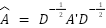
GCNs are based on encoding the graph data into matrices then plugging that data into convolutional layers, following a neural network architecture similar to others such as the LSTM.  The key insight is to encode the graph into a matrix built around the following equation:</p>

<p><img src="../assets/img/intro_graph_post/formula_one.png" alt="Matrix Formula" /></p>

<p>Where A’ is the normalized adjacency matrix and D is the diagonalization. A good walkthrough of the derivation for this formula can be found <a href="https://medium.com/@jrosseruk/demystifying-gcns-a-step-by-step-guide-to-building-a-graph-convolutional-network-layer-in-pytorch-09bf2e788a51">here</a>.</p>

<p>The original GCN paper then defined the forward layer using the formula</p>

<p><img src="../assets/img/intro_graph_post/formula_two.png" alt="Conv Layer Formula" /></p>

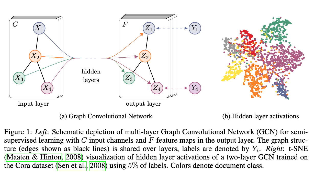
<p>The high level view of the system would then look like the diagram below, taken from the paper itself:<br />
<img src="../assets/img/intro_graph_post/GCN_diagram.png" alt="GCN Diagram" />
<a href="https://arxiv.org/pdf/1609.02907">Source</a></p>

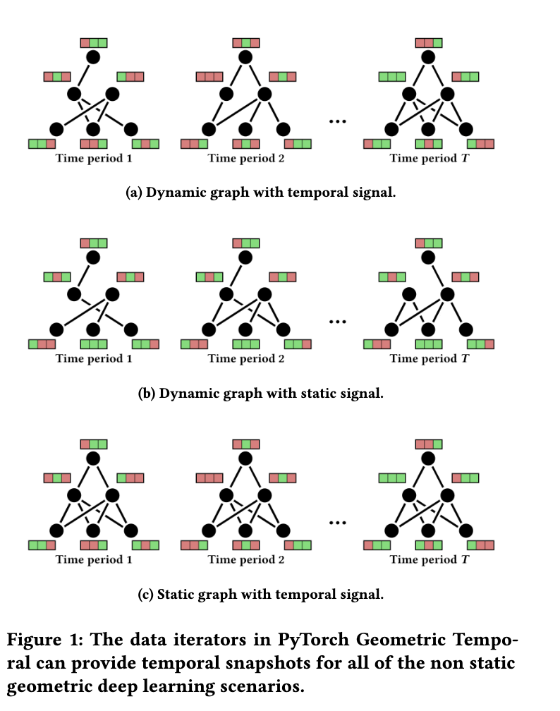
<p>In my work, we explored the use of GCNs for prediction tasks to forecast crop disease spread. To this end, we experimented with <a href="https://arxiv.org/pdf/2104.07788">STM-Graphs</a> (Spatio-Temporal Graphs), because our data consisted of a mix of historical data types, such as weather recordings, and spatial data types, such as road networks. Basically, these models split each historical reading into a separate node, then chain them together to incorporate the spatial information. An implementation using PyTorch Geometric can be found <a href="https://github.com/Ahghaffari/stm_graph">here</a>.</p>

<p><img src="../assets/img/intro_graph_post/STM_diagram.png" alt="STM Diagram" />
<a href="https://arxiv.org/pdf/2104.07788">Source</a></p>

<h1 id="closing-thoughts">Closing Thoughts</h1>

<p>This post was a brief look at graph models in machine learning and their potential use cases. Hopefully I’ll give some deeper dives in the near future, and maybe even present some example cases, so stay tuned!</p>]]></content><author><name></name></author><summary type="html"><![CDATA[In my previous post, I mentioned that I’ve been exploring the use of graph methods in modeling and deep learning, some for work and some for my own hobby projects. Because I spent much of September traveling and resting before starting a new grad program, I haven’t had a lot of time recently for diving more into this topic, but I wanted to put together a short post summarizing the things I’ve learned so far to lay the groundwork for future posts on graph models.]]></summary></entry><entry><title type="html">Gemma 4 12B and Methods of Multimodal Models</title><link href="/blog/multimodal_methods" rel="alternate" type="text/html" title="Gemma 4 12B and Methods of Multimodal Models" /><published>2026-08-31T00:00:00+00:00</published><updated>2026-08-31T00:00:00+00:00</updated><id>/blog/Multimodal-Methods</id><content type="html" xml:base="/blog/multimodal_methods"><![CDATA[<p>A few months ago, in June 2026, Google <a href="https://blog.google/innovation-and-ai/technology/developers-tools/introducing-gemma-4-12b/">released</a> their latest model in the Gemma 4 family: Gemma 4 12B. The Gemma family is Google’s set of open-source models, and this particular model release was designed to be smaller but still maintain a high level of performance. However, beyond its small size, this model is advertised as being “encoder-free”, while still retaining multimodal capabilities. Multimodal systems are those that process different ‘modalities’ of data (text, audio, visual, etc.) within the same system. <br />
Reading through the press releases led me to want to understand what exactly is meant by “encoder-free”; in the process, I ended up going through a large review of the methods multimodal systems use to incorporate different modalities into their systems. In some sense, many of my previous posts have already been focused on multimodal systems, since most of the audio generation systems and all of the text-to-speech systems handle both text and audio data. However, I haven’t explicitly covered the way these different data types are handled before. Thus, this post will look at the different strategies that can be used in developing a multimodal system, then will take a look at the way Gemma 4 approaches it and how it is different from previous approaches.</p>

<h1 id="multimodal-methods">Multimodal methods</h1>

<p>Researchers have experimented with many different ways to incorporate multiple data modalities into a complete system. I’m going to outline a number of the different methods I’ve come across, and I’ll try to point out any generative audio models we’ve seen before that use these methods. I’ll try to cover things in order of overall adoption, so the first few methods I’ll cover are used by the majority of multimodal systems. I’ll then highlight the difference in Gemma 4 12B; in particular, what it means to be “encoder-free”.</p>

<h2 id="separate-encoders">Separate Encoders</h2>

<p>Probably the most straightforward and widely-used method is to simply add a separate encoder for each modality then combine the resulting data together. Combining the data has two main approaches: appending the data together, or encoding the data then using a joint embedding space (an example of this would be CLIP).</p>

<p>A good example of this method is outlined in <a href="https://arxiv.org/pdf/2309.05519">NExT-GPT: Any-to-Any Multimodal LLM</a>, published June 2024. It uses separate encoders for the input modalities, followed by a LLM central router with semantic understanding and reasoning, and resulting in separate output projections<br />
From the paper, the LLM “outputs: 1) the textual responses directly, and 2) signal tokens of each modality that serve as instructions to dictate the decoding layers on whether to generate multimodal contents and what content to produce if yes”.</p>

<p>For a further modification to this method, the separate encoders can be connected to a shared parameter space down the line. An example of this is in the <a href="https://arxiv.org/pdf/2408.11039">Transfusion</a> paper from Meta, published August 2024. This model uses separate components with unshared parameters to embed the different modalities and different objective/loss functions for different modalities, but it maintains shared data parameters in the later layers. Additionally, marker tokens help separate the modalities.</p>

<p>The majority of generative audio models we’ve seen before make use of this method to handle the different modalities of text and audio, prominent examples including <a href="https://arxiv.org/pdf/2301.02111">VALL-E</a>, <a href="https://github.com/neonbjb/tortoise-tts">TorToiSE</a>, and <a href="https://llasatts.github.io/llasatts/">Llasa</a>.</p>

<h2 id="unified-architecture">Unified architecture</h2>

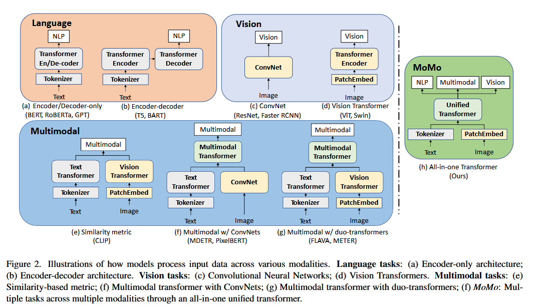
<p>For the next method, instead of using multiple encoders, some multimodal systems use a single encoder then pass the results to a shared latent space. These models typically make use of contrastive loss such as CLAP or CLIP. <br />
We can see this method in action in the <a href="https://arxiv.org/pdf/2304.05523">MoMo</a> paper, published in April 2023, which makes use of a single-stream encoder to process both text and image data.</p>

<p><img src="../assets/img/multimodal_post/momo_process.png" alt="momo_process" />
	<a href="https://arxiv.org/pdf/2304.05523">Source</a></p>

<p>Another good primer for how this method is implemented can be found in the paper <a href="https://arxiv.org/pdf/2503.01654">A Shared Encoder Approach to Multimodal Representation Learning</a>. Published in March 2025, this paper outlines a method of using additional information to mark the data types, so that the model can inherently learn what to do with the different data types. It appends a “modality feature vector” or token to the embedded data to give the encoder info on what data type it is.</p>

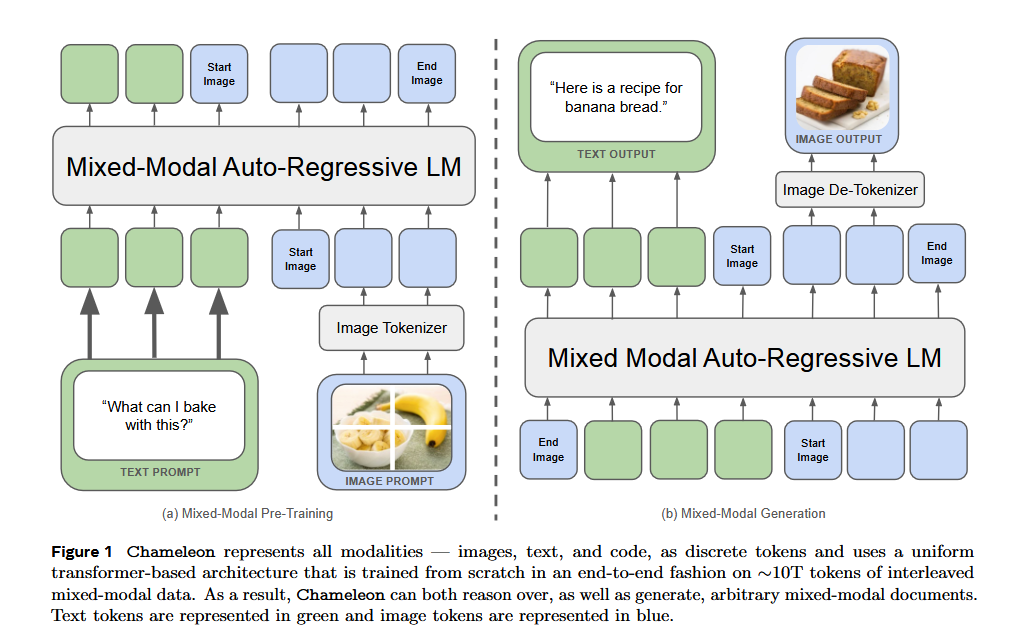
<p>A further example can be found in the <a href="https://arxiv.org/pdf/2405.09818">Chameleon</a>, published May 2024 from Meta.<br />
<img src="../assets/img/multimodal_post/chameleon_arch.png" alt="chameleon_arch" />
<a href="https://arxiv.org/pdf/2405.09818">Source</a></p>

<p>Of the audio models we’ve looked at before, the most relevant for this method is <a href="https://arxiv.org/html/2301.12503v3">AudioLDM</a>, which uses Contrastive Language-Audio Pretraining (CLAP) to align the text and audio embeddings into a joint cross-modal space.</p>

<h2 id="cross-modal-attention">Cross-modal attention</h2>

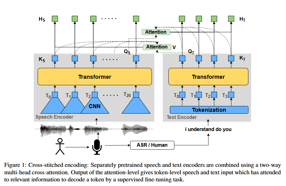
<p>The next method handles different data modalities not in the initial data encoder but within the attention process. <a href="https://www.emergentmind.com/topics/cross-modal-attention">Cross-Modal Attention Mechanisms</a> compute dependencies across different data modalities “by selectively conditioning the representation of one modality on features from another”. Essentially, this method uses the self-attention paradigm, but query values in modality1 attend to keys and values in modality2. Attention in these systems can be bidirectional, hierarchical, or single- or multi-headed.</p>

<p>This method is harder to implement so it doesn’t get used quite as much, but it has still seen an abundance of research directed toward it. One example is in the paper <a href="https://arxiv.org/pdf/2204.09227">Cross-stitched Multi-modal Encoders</a> from April 2022. The developers here combine speech and text encoders using a jointly trained attention mechanism. They use a pretrained Wav2vec2 model for turning the audio segments into embeddings and a pretrained text encoder for text token embeddings, then pass the different embeddings into the multi-head attention.<br />
<img src="../assets/img/multimodal_post/cross_modal_attn.png" alt="cross_modal_attn" /><br />
<a href="https://arxiv.org/pdf/2204.09227">Source</a></p>

<h2 id="mixture-of-experts">Mixture of Experts</h2>

<p>Moving into the realm of less-frequently used but still very interesting methods, some researchers have experimented with using Mixture of Experts (MoE) models to actually use the “experts” for handling the different data modalities.</p>

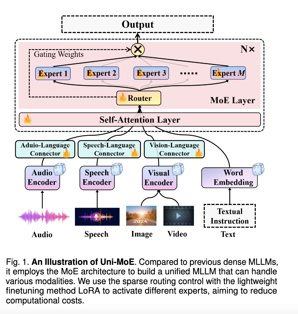
<p>The paper <a href="https://arxiv.org/pdf/2405.11273">Uni-MoE: Scaling Unified Multimodal LLMs with Mixture of Experts</a>, published May 2024, uses modality-specific encoders with connectors for a unified multimodal representation followed by sparse MoE architecture with modality-specific experts. It uses an expert “router” to determine which expert to send the input to taking modality into account.<br />
<img src="../assets/img/multimodal_post/uni_moe_arch.png" alt="uni_moe_arch" /><br />
<a href="https://arxiv.org/pdf/2405.11273">Source</a></p>

<p>For another variation of the MoE method, the paper <a href="http://arxiv.org/html/2502.15381v1">MOVE: A Mixture-of-Vision-Encoders Approach for Domain-Focused Vision-Language Processing</a> from February 2025 moves the MoE aspect further up the pipeline by setting up multiple encoders for images (e.g. high-resolution vs low-resolution) and using an expert router to determine which encoder to use. In this sense it is actually a bit of a hybrid, using both separate modal encoders as well as MoE</p>

<h2 id="graph-approaches">Graph Approaches</h2>

<p>The final method I’ll highlight is to encode the various modalities and incorporate them into a graph model. The paper “<a href="https://arxiv.org/pdf/2007.08742">A Novel Graph-based Multi-modal Fusion Encoder for Neural Machine Translation</a>” explains this approach. It builds unified a graph to represent the input sentence and image, with the goal of capturing semantic relationships. This is using a graph network to guide the separate embedders and attention, acting in a way like separate encoders, but it also uses cross-modal gating, in a way similar to cross-attention, to connect the semantic relationships and complete the encoding process.</p>

<p>I’ve been exploring graph models a bit more lately, and I may dive deeper into the topic in a future post, so stay tuned.</p>

<h2 id="gemma-4-12b">Gemma 4 12B</h2>

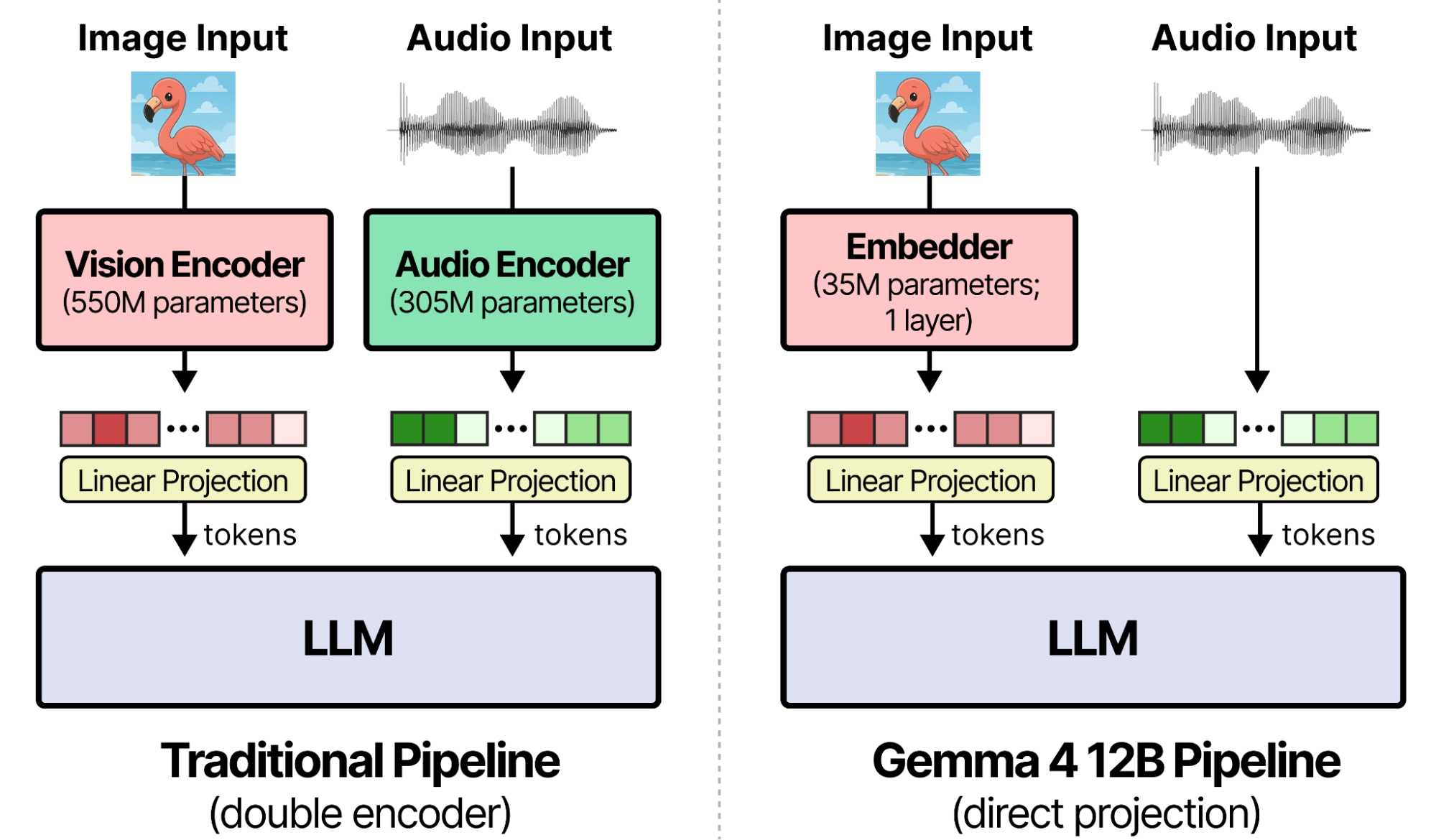
<p>Now that we’ve covered the main ways researchers have thus far focused on building out multimodal systems, we can finally get to the model that helped inspire this post: Gemma 4 12B. So what is it doing and how is it different? Well, the system looks very similar to the separate encoders method, because each modality is processed in its own module. However, instead of an encoder, which is a multi-layer neural net that has to be trained and tuned, the modules are merely embedding matrices. From the <a href="https://blog.google/innovation-and-ai/technology/developers-tools/introducing-gemma-4-12b/">release</a>:</p>

<ul>
  <li><strong>Vision:</strong> We replaced Gemma 4’s vision encoder with a lightweight embedding module consisting of a single matrix multiplication, positional embedding and normalizations. This allows the LLM backbone to take over visual processing.</li>
  <li><strong>Audio:</strong> We simplified audio processing even further. We removed the audio encoder entirely and projected the raw audio signal into the same dimensional space as text tokens.</li>
</ul>

<p>What happens is that the image data is passed through a very simple embedding function that maps the pixel data to a linear space, while the audio data is sliced into 40ms clips and projected linearly as well. The data is then all tossed into the LLM, a decoder-only Transformer, to do the heavy lifting of interpretation and generation.</p>

<p><img src="../assets/img/multimodal_post/gemm412b.png" alt="gemm412b" /><br />
<a href="https://developers.googleblog.com/gemma-4-12b-the-developer-guide/">Source</a></p>

<p>The result is a much smaller model, because it uses a single-layer (35M parameter) vision embedder when previously it would have used a multi-layer vision encoder (multi-billion parameter) from a transformer.</p>

<p>This is a very brief summary of what the model is doing. If you’d like more detail, an in-depth guide detailing extra information such as the incorporation of positional information in the vision tokens using X and Y coordinate matrices can be found <a href="https://newsletter.maartengrootendorst.com/p/a-visual-guide-to-gemma-4-12b">here</a>. In a sense the model is intensively simplifying the data transformation process and letting the LLM figure out the data modality info on its own, but the results show that this is still able to work remarkably well.</p>

<h1 id="closing-thoughts">Closing Thoughts</h1>

<p>So there you have it: the different ways researchers have built systems to process multiple data modalities, as well as a new interesting approach from Google. Technically speaking, the encoder-free method isn’t completely novel, as stripping out the encoder from vision-language models has been explored in <a href="https://github.com/baaivision/EVE">other places</a> as well, but Google has certainly pushed the frontier in the development and incorporation of the technique.<br />
If you’d like to dive even deeper into this topic, some interesting papers to look at are: <a href="https://arxiv.org/pdf/2306.13549">A Survey on Multimodal Large Language Models</a>, a November 2024 paper that explores the module components of multimodal LLMs ; and <a href="https://www.techrxiv.org/doi/pdf/10.36227/techrxiv.176289261.16802577/v1">A Survey of Unified Multimodal Understanding and Generation: Advances and Challenges</a>, an October 2025 survey of over 700 papers involving multimodal systems, which attempts to categorize different themes and trends seen in the research community.</p>]]></content><author><name></name></author><summary type="html"><![CDATA[A few months ago, in June 2026, Google released their latest model in the Gemma 4 family: Gemma 4 12B. The Gemma family is Google’s set of open-source models, and this particular model release was designed to be smaller but still maintain a high level of performance. However, beyond its small size, this model is advertised as being “encoder-free”, while still retaining multimodal capabilities. Multimodal systems are those that process different ‘modalities’ of data (text, audio, visual, etc.) within the same system. Reading through the press releases led me to want to understand what exactly is meant by “encoder-free”; in the process, I ended up going through a large review of the methods multimodal systems use to incorporate different modalities into their systems. In some sense, many of my previous posts have already been focused on multimodal systems, since most of the audio generation systems and all of the text-to-speech systems handle both text and audio data. However, I haven’t explicitly covered the way these different data types are handled before. Thus, this post will look at the different strategies that can be used in developing a multimodal system, then will take a look at the way Gemma 4 approaches it and how it is different from previous approaches.]]></summary></entry><entry><title type="html">Vector Quantization and Continous Codes in Audio ML</title><link href="/blog/vq_cont_codes" rel="alternate" type="text/html" title="Vector Quantization and Continous Codes in Audio ML" /><published>2026-07-18T00:00:00+00:00</published><updated>2026-07-18T00:00:00+00:00</updated><id>/blog/vq-cont-codes</id><content type="html" xml:base="/blog/vq_cont_codes"><![CDATA[<p>Quantization has become highly <a href="https://developer.nvidia.com/blog/model-quantization-concepts-methods-and-why-it-matters/">incorporated across the range</a> of Machine Learning and GenAI use cases. Aimed at finding gains in storage and computational efficiency, this method is largely used in systems that deal with image and audio data classification and generation, although potential use cases exist in other areas such as <a href="https://medium.com/@waleed.physics/the-future-of-time-series-modeling-tokenization-through-vector-quantization-77ed3bc745d8">time series</a>. Quantization helps to reduce memory requirements and speeds up computation, while trading off some level of accuracy.</p>

<p>It is important to realize though that depending on context quantization may be applied to different parts of the machine learning pipeline. I hear it used most often in the context of quantization of weights, where the format of model parameters are reduced to lower-precision values, e.g. from FP32 to FP8. Quantization of weights typically involves some rounding and/or clippling around a “zero point”, as well as decisions around how much of the parameter space you want to quantize and when you want quantization to take place in the training process. Broadly speaking, you have two options: PTQ and QAT. Post-training quantization (PTQ) takes place after the training has occurred, whereas <a href="https://www.ibm.com/think/topics/quantization-aware-training">Quantization-Aware Training</a> (QAT) is incorporated into the training process.</p>

<p>Another important context though where quantization gets applied is in the data itself. Because we work with data of such large quantities and shapes, methods have been developed to quantize the data for use during training and inference. We’ve actually seen this concept before, when we took a look at <a href="https://8t88.github.io/blog/latent_space_neural_codecs">audio codecs</a>. In this post I want to dive deeper into the process of what data quantization actually looks like, highlighting the pros and cons to this tool, and also take a look at a possible alternative. As before, I’ll explore these ideas with my favorite use case: audio generation.</p>

<h2 id="vector-quantization-in-audio-codecs">Vector Quantization in Audio Codecs</h2>

<h3 id="codec-refresher">Codec Refresher</h3>

<p>As a quick review, an audio codec is a system that compresses the information contained in audio data (i.e. the waveform) into latent space. The results of this compression are called “codes”.<br />
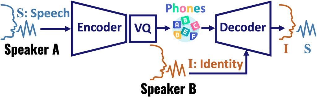
Vector Quantization (VQ) forms a key component of the codec. In our real-world example, <a href="https://arxiv.org/pdf/2107.03312">SoundStream</a> runs the audio waveform through an encoder then applies Residual Vector Quantization (RVQ) to the encoded audio data, after which the result is run through the decoder, thus producing the audio tokens. <br />
So the overall process looks like: continuous data inputs get translated into continuous latent representations, then the quantization maps continuous latent representations into discrete embeddings before being further transformed. This process is incorporated into the overall machine learning pipeline that generates audio, as the below picture illustrates.</p>

<p><img src="../assets/img/vq_post/vq_arch.png" alt="vq_in_audio_ml" width="50%" /></p>

<p><a href="https://towardsdatascience.com/interpretable-latent-spaces-using-space-filling-vector-quantization-e4eb26691b14/">source</a></p>

<h3 id="quantization-processes">Quantization Processes</h3>

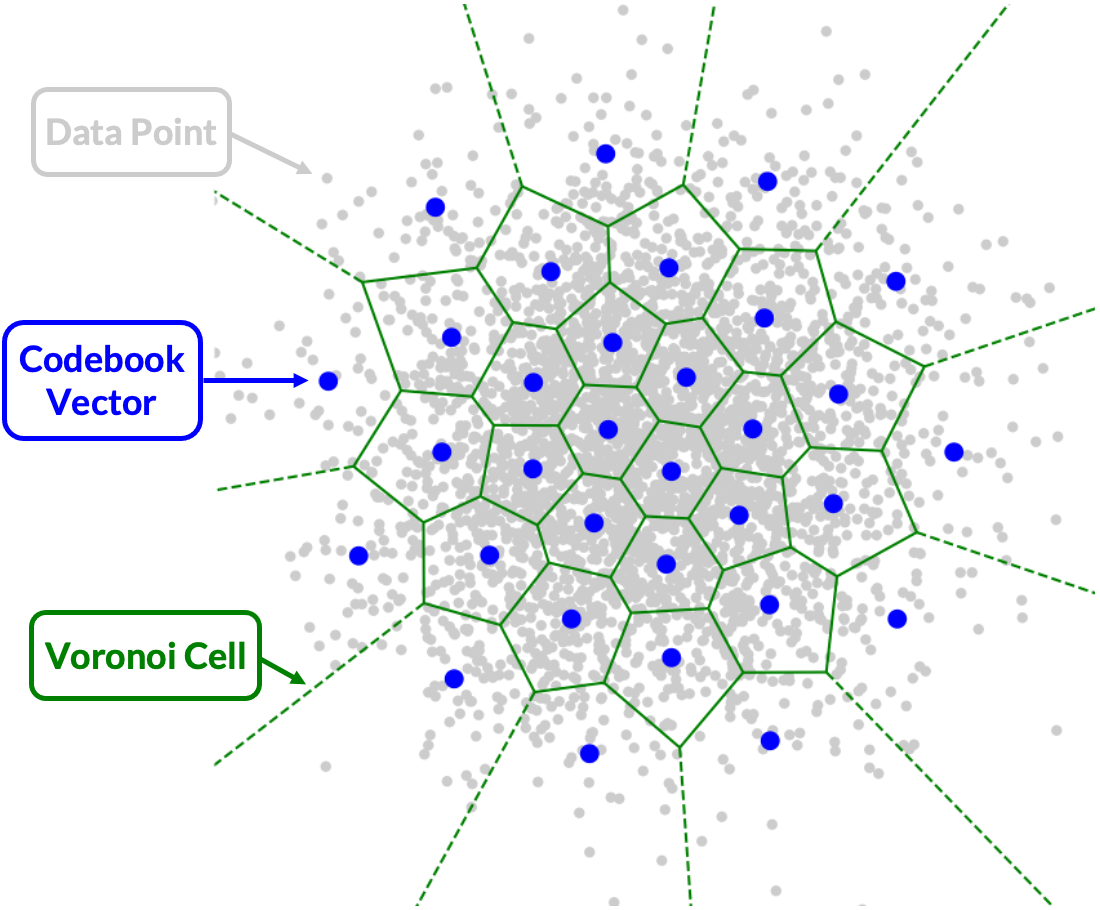
<p>So what does the mechanism of Vector Quantization actually look like? This is a different process from the quantization used for model parameters. In the data quantization context we are not simply truncating the precision; instead, we are trying to map each data point to the closest low-precision value by using a distance function to calculate the space between data which is typically very high-dimensional, thus maintaining a semantic accuracy while achieving data compression,. VQ commonly uses clustering methods such as K-means to cluster similar parts of the spectrogram. It then maps these clustered data points to the nearest codebook point. <br />
A codebook is a collection of representative vectors (codewords), and each input feature vector is assigned to the nearest codeword in the codebook. The index of the assigned codeword in the codebook then becomes a discrete token.</p>

<p><img src="../assets/img/vq_post/codebook_diagram.png" alt="codebook_diagram" width="75%" /></p>

<p><a href="https://towardsdatascience.com/interpretable-latent-spaces-using-space-filling-vector-quantization-e4eb26691b14/">source</a></p>

<p>If you want to examine the finer details of vector-quantization, <a href="https://github.com/lucidrains/vector-quantize-pytorch">this</a> repo provides examples of the different implementations. Furthermore, <a href="https://huggingface.co/blog/ariG23498/understand-vq">this</a> post from Hugging Face gives a good walkthrough of the steps involved in quantization, showing the process of flattening, computing distance, and selecting the closest codebook vector.</p>

<h3 id="vq-varieties">VQ Varieties</h3>

<p>There are many different types of vector quantization methods; some of the most well-studied include:</p>

<ul>
  <li>Residual Vector Quantization (RVQ): A technique that approximates high-dimensional vectors by selecting elements from a series of dictionaries, iteratively minimizing the quantization error</li>
  <li>Linde-Buzo-Gray (LBG) algorithm: A popular method for designing codebooks using a hierarchical clustering approach</li>
  <li>Generalized Residual Vector Quantization (GRVQ): An improved version of RVQ that demonstrates better performance in terms of quantization accuracy and computational efficiency</li>
  <li>Improved Residual Vector Quantization (IRVQ): Another improved version of RVQ that further enhances its performance</li>
</ul>

<p><a href="https://www.activeloop.ai/resources/glossary/residual-vector-quantization/">This</a> blog post dives into the specifics of these different types of vector quantization, and provides useful illustrations</p>

<p>RVW, the method SoundStream uses, has been around for <a href="https://ieeexplore.ieee.org/abstract/document/480761">decades</a>, but its incorporation into Generative AI was made popular with <a href="https://arxiv.org/abs/1711.00937">VQ-VAE</a>, a model introduced in the paper “<a href="https://proceedings.neurips.cc/paper/2017/file/7a98af17e63a0ac09ce2e96d03992fbc-Paper.pdf">Neural Discrete representation Learning</a>” by Oord et al.<br />
RVQ works by iteratively minimizing the quantization error, which is the difference between the original vector and its approximation.</p>

<p><img src="../assets/img/vq_post/rvq_diagram.png" alt="rvq_diagram" /> <br />
	<a href="https://medium.com/data-science/optimizing-vector-quantization-methods-by-machine-learning-algorithms-77c436d0749d">source</a></p>

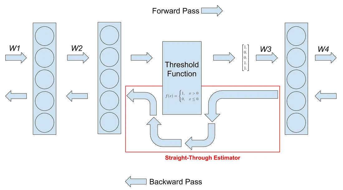
<p>To incorporate RVQ into your deep learning model, you need a trick to complete backpropagation, since the quantization doesn’t have a gradient. A key insight of VQ-VAE, which allowed the model to actually get trained, was the Straight-through estimator (STE) identified in the diagram below. STE calculates the gradient for each layer and passes it back by skipping over the quantization function.</p>

<p><img src="../assets/img/vq_post/ste_diagram.png" alt="ste_diagram" /><br />
<a href="https://hassanaskary.medium.com/intuitive-explanation-of-straight-through-estimators-with-pytorch-implementation-71d99d25d9d0">source</a></p>

<p>If you want to dive even deeper, some other interesting VQ methods to learn about are:</p>

<ul>
  <li><a href="https://medium.com/data-science/improving-vector-quantization-in-vector-quantized-variational-autoencoders-vq-vae-915f5814b5ce">Noise Substitution in Vector Quantization for Machine Learning (NSVQ)</a>: “a technique in which the vector quantization error is simulated by adding noise to the input vector, such that the simulated noise would gain the shape of original VQ error distribution.“</li>
  <li><a href="https://towardsdatascience.com/interpretable-latent-spaces-using-space-filling-vector-quantization-e4eb26691b14/">Space-Filling Vector Quantization (SFVQ)</a>: “mapping input data points on a space-filling curve (rather than only mapping data points exclusively on codebook vectors as what we do in normal VQ) “</li>
</ul>

<h2 id="continuous-tokens">Continuous Tokens</h2>

<p>As a refresher, there are a few different options for audio generation system architectures:</p>

<ul>
  <li>Transformer architecture on discrete audio tokens; incorporating the VQ methods we talked about above; used by systems such as <a href="https://arxiv.org/abs/2506.21619">IndexTTS2</a></li>
  <li>Diffusion model; examples include <a href="https://arxiv.org/pdf/2308.05734">AudioLDM 2</a>, as well as <a href="https://arxiv.org/pdf/2404.09956">Tango 2</a>, which is coupled with the decoder of a VAE (turning the latent representation to a mel-spectrogram) followed by a vocoder to produce the waveform</li>
  <li>Auto-regressive Transformer on continuous audio tokens, where the diffusion aspect is used to model the continuous token then the transformer predicts the next continuous token</li>
</ul>

<p>As you likely know, the general idea of LLMs were based on autoregressive models applied to discrete space, i.e. language and vocabulary. These systems were then applied on image space, despite it being more of a continuous domain. To accomplish this, the data would be vector-quantized and fed into a next-token predictor.<br />
However, if we didn’t want to use VQ to produce discrete tokens to be used in the generative audio models, what would continuous tokens in audio ML, i.e. the third option, look like?</p>

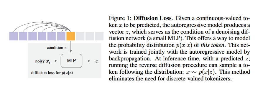
<p>The paper <a href="https://arxiv.org/pdf/2406.11838">Autoregressive Image Generation without Vector Quantization</a> lays out a method to apply autoregressive models in a continuous-valued space (in this case image data) by modeling the per-token probability distribution using a diffusion procedure. This paper points out that the basic autoregressive idea of “predicting next tokens based on previous ones”  does not depend on predicting values that are continuous. Instead, all you really need is a loss function and a sampler. The loss function measures the per-token probability distribution, which is used to build model distributions to be sampled. Discrete-valued representations are convenient in this instance because they can be modeled by a categorical distribution using cross-entropy loss and sampling based on softmax. To apply this to the continuous domain though, the paper instead uses a Diffusion Loss function  (in the score matching sense) to model the per-token probability and samples from the resulting distribution. The system predicts a vector for each token, which is then fed into a diffusion model as a conditioning vector to guide the model. Thus the input and target can be continuous-valued data.</p>

<p><img src="../assets/img/vq_post/diffusion_loss_cc.png" alt="diffusion_loss_cc" /><br />
			<a href="https://arxiv.org/pdf/2406.11838">source</a></p>

<p>The paper also combines standard autoregressive models and masked generative models into a general framework wherein the masked autoregressive models “ predict multiple output tokens simultaneously in a randomized order, while still maintaining the autoregressive nature of “predicting next tokens based on known ones” …  This leads to a masked autoregressive (MAR) model that can be seamlessly used with Diffusion Loss.“</p>

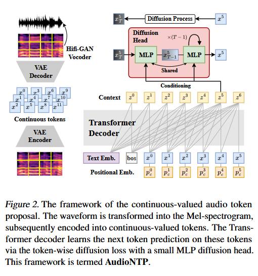
<p>Using these concepts, we can apply the idea to the continuous data in the audio domain.  The paper <a href="https://arxiv.org/pdf/2507.09834">Generative Audio Language Modeling with Continuous-valued Tokens and Masked Next-Token Prediction</a> does just that; it took inspiration from the image generation paper above and applied similar ideas on audio data. The paper sets up a pre-processing pipeline based on AudioLDM to feed the Mel-spectogram of the audio batch into the encoder of the VAE, with a few additional transformations to produce continuous-valued tokens with the latent size 128. The pipeline used this latent representation to predict the next-token using a Transformer decoder token-wise diffusion loss with a small MLP diffusion head.<br />
<img src="../assets/img/vq_post/audioNTP_diagram.png" alt="audioNTP_diagram" /><br />
				<a href="https://arxiv.org/pdf/2507.09834">source</a><br />
During inference, the predicted next-tokens are decoded back into a Mel-spectrogram, then converted to an audio file with a vocoder. <br />
The final result: use a transformer to predict next-token, but the tokens are continuous, and diffusion loss is used to work with those continuous tokens</p>

<h2 id="continuous-codes-advantages">Continuous Codes Advantages</h2>

<p>As a final thought, you may be asking: why would we want to do this?<br />
Continuous tokens help to counter the downsides of information loss that comes as a natural side effect of quantization. Moreover, they maintain the benefits that tokenization brings of smaller and faster models coupled with the inherent streaming capabilities. Additionally, the downside of processes like RVQ is that the multiple steps of the VQ process make the pipeline scale in complexity and computation cost; an architecture based on continuous tokens may avoid this.</p>

<p>The idea of using continuous codes holds many potential advantages, but it is still in a research state and has not been heavily incorporated into existing audio generation systems. For the time being, Vector Quantization remains a vital tool to allow ML systems to effectively handle and model the type of giant datasets that come with audio.</p>]]></content><author><name></name></author><summary type="html"><![CDATA[Quantization has become highly incorporated across the range of Machine Learning and GenAI use cases. Aimed at finding gains in storage and computational efficiency, this method is largely used in systems that deal with image and audio data classification and generation, although potential use cases exist in other areas such as time series. Quantization helps to reduce memory requirements and speeds up computation, while trading off some level of accuracy. It is important to realize though that depending on context quantization may be applied to different parts of the machine learning pipeline. I hear it used most often in the context of quantization of weights, where the format of model parameters are reduced to lower-precision values, e.g. from FP32 to FP8. Quantization of weights typically involves some rounding and/or clippling around a “zero point”, as well as decisions around how much of the parameter space you want to quantize and when you want quantization to take place in the training process. Broadly speaking, you have two options: PTQ and QAT. Post-training quantization (PTQ) takes place after the training has occurred, whereas Quantization-Aware Training (QAT) is incorporated into the training process.]]></summary></entry><entry><title type="html">Transformer and Diffusion models, and their role in audio generation</title><link href="/blog/transform_diffus_models_audio_gen" rel="alternate" type="text/html" title="Transformer and Diffusion models, and their role in audio generation" /><published>2026-04-09T00:00:00+00:00</published><updated>2026-04-09T00:00:00+00:00</updated><id>/blog/transform-diffus-models-audio-gen</id><content type="html" xml:base="/blog/transform_diffus_models_audio_gen"><![CDATA[<p>Much has been written about the different categories of <a href="https://deepgenerativemodels.github.io/notes/">generative models</a>: VAEs, GANs, flow-based models, etc. Since 2022, the two types of generative models I seem to hear most frequently discussed are Transformers and Diffusion models. These two models made headlines because ChatGPT was powered by transformers and DALL-E 2 (as well as Stable Diffusion) was powered by diffusion. However, in reading about these models, I had a bit of a tough time understanding how exactly transformers differ from diffusion models. After all, they seem to rely on the same fundamental concepts of encoding and decoding. Furthermore, like I mentioned in a previous <a href="https://8t88.github.io/blog/tts_arch_trends">post</a>, some audio generation systems such as <a href="https://github.com/neonbjb/tortoise-tts">TorToise</a> incorporate both these types of models. So, is there a sharp distinction between the two? The answer, as it turns out, is that the two are indeed distinct, but they can overlap if the architecture of the diffusion model uses the transformer as a backbone. <br />
While I won’t dive into the low-level mathematical details of how these two models work, given that others have <a href="https://yang-song.net/blog/2021/score/">already</a> <a href="https://angusturner.github.io/generative_models/2021/06/29/diffusion-probabilistic-models-I.html">done</a> <a href="https://benanne.github.io/2022/01/31/diffusion.html">so</a> with far greater depth and insight than I could, in this post I will highlight the key conceptual insight I think provides a meaningful distinction, that of denoising. Additionally, I will take a look at the specifics of how this implementation plays out by exploring some generative audio systems that make use of diffusion and transformer components, pointing out where and how each is implemented to help make the difference more concrete.</p>

<h2 id="quick-overview">Quick Overview</h2>

<h3 id="transformers">Transformers</h3>

<p>At this point, most of us have at least some familiarity with the transformer. It is a neural network architecture that relies on data embedding, an encoder and/or decoder, and some form of attention. The Transformer was initially set out in a 2017 paper and used an autoencoder structure, but the systems that really brought the transformer acclaim, the GPT family, are decoder-only systems. Andrej Karpathy’s <a href="https://github.com/karpathy/nanogpt">nanoGPT</a> is an easy reference for understanding this: we see that the layers are feedforward + attention, without an initial encoding of the embedded text data. These text-generating models predict sequences that follow an initial prompt</p>

<h3 id="diffusion">Diffusion</h3>

<p>Diffusion models, sometimes called score-based models, are a class of generative models that learn to reverse a ‘forward’ process of adding noise to a dataset. They were outlined in a <a href="https://arxiv.org/abs/1711.05772v2">2015 paper</a> but got a lot more attention five years later from the paper <a href="https://arxiv.org/abs/2006.11239v2">Denoising Diffusion Probabilistic Models</a>. <br />
Diffusion models also use an encoding/decoding structure to transform the input. The 2020 paper used a U-Net for this. During inference, the U-Net takes as input either an image (in the case of the original denoising diffusion models paper) or a latent encoded image (as in <a href="https://arxiv.org/abs/2112.10752">latent diffusion</a>) and outputs the predicted noise. This predicted noise is then subtracted from the input to get a slightly less noisy image; that process is repeated a number of times before passing the result to the decoder to get the final image output.<br />
To really understand diffusion models, I’d recommend <a href="https://towardsdatascience.com/the-art-of-noise/">this</a> in-depth walkthrough of the implementation of a diffusion model with a U-net, as well as <a href="https://colab.research.google.com/gist/anton-l/f3a8206dae4125b93f05b1f5f703191d/diffusers_training_example.ipynb#scrollTo=584739c5-83f5-4077-8379-89a7c9ff1bf2">this</a> colab notebook. An important point, which took me a while to realize, is that the U-Net gets run during each step, rather than each step representing a layer of the U-Net, as this <a href="https://raw.githubusercontent.com/patrickvonplaten/scientific_images/master/stable_diffusion.png">diagram</a> illustrates. Also as a brief aside, diffusion models don’t simply predict as much noise as possible and remove it during each step. Instead, they use noise schedulers to control the rate this is performed. You can find a good writeup of that <a href="https://medium.com/@lambdafluxofficial/developers-guide-to-hugging-face-diffusers-part-3-deep-dive-into-scheduler-e88fe2371b74">here</a>, as well as a detailed notebook walkthrough <a href="https://colab.research.google.com/github/huggingface/notebooks/blob/main/diffusers/diffusers_intro.ipynb#scrollTo=RwSsSoRVY136">here</a>.</p>

<h2 id="key-difference-denoising">Key Difference: Denoising</h2>

<p>Now that we’ve given a high-level overview of what these two models are, we can identify the key aspect that separates a diffusion model from a standard transformer.<br />
Looking at the output of the system, we realize that the transformer model isn’t necessarily trying to predict noise, it is trying to predict the next token in a sequence. For the GPT series, this was focused on language, thus the training set consisted of for example wikipedia articles. The training process started with a sentence and the model tried to predict the next word in the sentence, with the loss comparing how close the prediction is to the actual next word.<br />
For diffusion models, however, the prediction aspect of the model isn’t actually the result. Instead, the prediction within the model is noise, which is used in the denoising module to generate the output. In other words, the noise is predicted within the system, then that prediction is used to produce the final output, whether that’s an image, audio clip, etc. The difference is a bit subtle but significant.</p>

<h2 id="overlap">Overlap</h2>

<p>Denoising is necessary for a diffusion model, but that doesn’t mean that the two models are mutually exclusive. In the initial paper, the diffusion model relies on a U-Net for its backbone, which is a convolutional neural network that takes in the image and downsamples then upsamples the data. However, <a href="https://lilianweng.github.io/posts/2021-07-11-diffusion-models/#model-architecture">as has been pointed out,</a> diffusion models can instead use the transformer as a backbone. This happens when attention is added in between the layers, making the transformer (embedding through convolutions followed by attention) the backbone of the model.<br />
This architecture setup is known as a <a href="https://arxiv.org/abs/2212.09748">Diffusion-transformer</a> (DiT). A <a href="https://encord.com/blog/diffusion-models-with-transformers/">DiT</a> uses transformers in a latent diffusion process, where a simple prior (like Gaussian noise) is gradually transformed into the target image. Stable Diffusion 3 uses a DiT, as seen in this <a href="https://i.imgur.com/D9y0fWF.png">diagram</a>.</p>

<h2 id="implementation-in-tortoise-and-indextts2">Implementation in TorToise and IndexTTS2</h2>

<p>Let’s look at some real-world examples by using one of my favorite ML topics: audio generation.</p>

<h3 id="tortoise">Tortoise</h3>

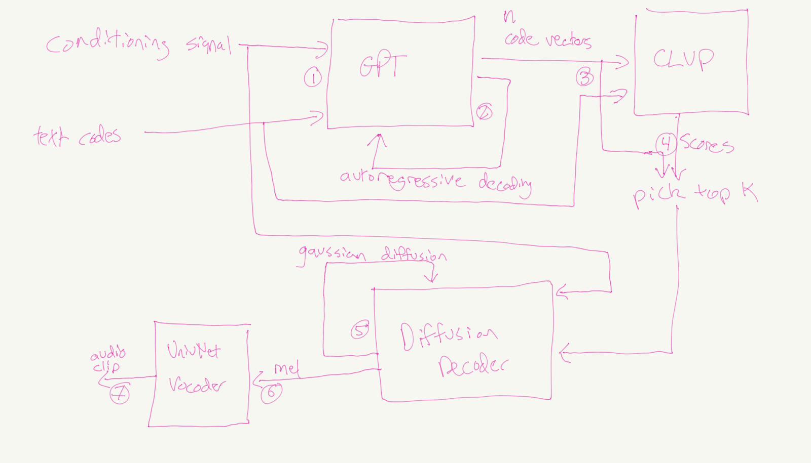
<p><img src="../assets/img/transform_diffus_post/tortoise_arch.png" alt="tortoise_architecture" /><br />
From the TorToise <a href="https://nonint.com/2022/04/25/tortoise-architectural-design-doc/">design doc</a></p>

<p>We’ll first take a look at <a href="https://arxiv.org/pdf/2305.07243">TorToise</a>, an audio generation text-to-speech system released in 2023. <br />
As described in the paper, TorToise takes the advances made by image generation in autoregressive transformers and DDPMs and applies them to speech synthesis. In this we find an example of when the transformer and diffusion models are separate, as you can see in the architecture drawing above. The transformer first predicts audio codes, then the diffuser generates spectrograms from the codes. So what does this implementation look like?<br />
TorToise uses a transformer to create speech tokens from the encoded speech and text inputs, resulting in “a probabilistic understanding of how text and speech relate to one another given a contextual voice”. It then uses a Diffusion model to decode the compressed speech representations into a wave file. Rather than using a U-net, the diffusion model “is composed of a flat stack of 10 alternating full-attention layers and residual conv blocks. The hidden dimensionality is 1024 with 16 attention heads. This model clocks in at 292M parameters.” (There are three other models in the TorToise system, but we are only focusing on these two for now.)</p>

<h3 id="indextts2">IndexTTS2</h3>

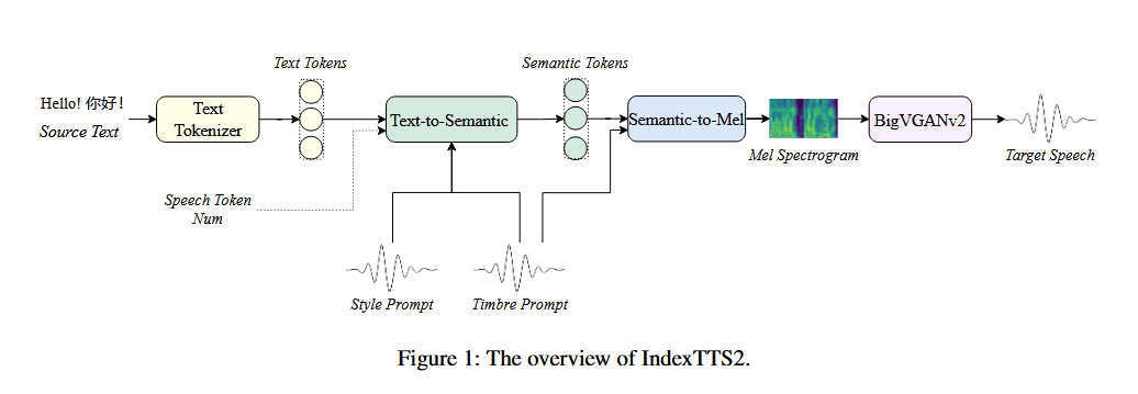
<p><img src="../assets/img/transform_diffus_post/indextts2_arch.png" alt="indextts2_architecture" /><br />
<a href="https://arxiv.org/pdf/2506.21619">Source</a></p>

<p><a href="https://arxiv.org/abs/2506.21619">IndexTTS2</a> (2025) is another high-quality text-to-speech system that has a particular focus on controlling speech duration and on achieving independent control over timbre and emotion. The model comprises three core modules: the Text-to-Semantic (T2S) module, the Semantic-to-Mel (S2M) module, and the Vocoder.<br />
The T2S module uses an autoregressive transformer framework to “generate semantic tokens from text, timbre/style prompts, and an optional speech token count”. The S2M module uses flow-matching modeling to sample from a noise distribution for generating mel-spectrograms. Flow-matching also transforms noise into structured data, though the method is a bit different from denoising diffusion models. We won’t go into detail here, but <a href="https://harshm121.medium.com/flow-matching-vs-diffusion-79578a16c510">this article</a> provides a good comparison between the two. <br />
You can see the IndexTTS team’s flow-matching implementation in their repo <a href="https://github.com/index-tts/index-tts/blob/main/indextts/s2mel/modules/flow_matching.py">here</a>; additionally, you should also note their <a href="https://github.com/index-tts/index-tts/blob/main/indextts/s2mel/modules/diffusion_transformer.py">implementation</a> of a diffusion transformer, which could presumably be substituted for the flow-matching module.</p>

<h2 id="final-thoughts">Final Thoughts</h2>

<p>Transformers and Diffusion models both incorporate the advances in machine learning around latent spaces, encoding/decoding, and attention. Their design and implementation are typically dictated by the nature of the task they are trying to accomplish. Diffusion models are excellent at synthesizing high-fidelity visual and auditory outputs, while transformers thrive on modeling and predicting sequential data. Sometimes though, as seen in the use cases above, combining the two produces a very powerful combination that results in the incredible realism of the generated text, audio, and video we see today.</p>]]></content><author><name></name></author><summary type="html"><![CDATA[Much has been written about the different categories of generative models: VAEs, GANs, flow-based models, etc. Since 2022, the two types of generative models I seem to hear most frequently discussed are Transformers and Diffusion models. These two models made headlines because ChatGPT was powered by transformers and DALL-E 2 (as well as Stable Diffusion) was powered by diffusion. However, in reading about these models, I had a bit of a tough time understanding how exactly transformers differ from diffusion models. After all, they seem to rely on the same fundamental concepts of encoding and decoding. Furthermore, like I mentioned in a previous post, some audio generation systems such as TorToise incorporate both these types of models. So, is there a sharp distinction between the two? The answer, as it turns out, is that the two are indeed distinct, but they can overlap if the architecture of the diffusion model uses the transformer as a backbone. While I won’t dive into the low-level mathematical details of how these two models work, given that others have already done so with far greater depth and insight than I could, in this post I will highlight the key conceptual insight I think provides a meaningful distinction, that of denoising. Additionally, I will take a look at the specifics of how this implementation plays out by exploring some generative audio systems that make use of diffusion and transformer components, pointing out where and how each is implemented to help make the difference more concrete.]]></summary></entry><entry><title type="html">Latent Spaces and Neural Codecs in Generative Audio</title><link href="/blog/latent_space_neural_codecs" rel="alternate" type="text/html" title="Latent Spaces and Neural Codecs in Generative Audio" /><published>2026-03-09T00:00:00+00:00</published><updated>2026-03-09T00:00:00+00:00</updated><id>/blog/latent-spaces-neural-codecs</id><content type="html" xml:base="/blog/latent_space_neural_codecs"><![CDATA[<p>As I mentioned in my <a href="https://8t88.github.io/blog/tts_arch_trends">last post</a>, one of the big developments in TTS architecture was the shift toward text to speech as a language modeling task with the use of audio tokens in the modeling process. In this post we’re going to dive into what that actually means and looks like in practice. We’ll start by giving a little bit of background looking briefly at the uses of latent spaces in earlier neural architectures. We’ll then see how latent spaces were applied to the audio domain, and we’ll take a closer look at the use of audio codes in this regard.<br />
So to begin, let’s explain what we mean by “latent spaces”.</p>

<h1 id="latent-spaces-and-encoders">Latent Spaces and Encoders</h1>

<p>A <a href="https://www.ibm.com/think/topics/latent-space">Latent space</a> is “a compressed representation of data points that preserves only essential features that inform the input data’s underlying structure”. These representations have been increasingly used in deep learning models over the last decade with the goal of teaching a model to capture information by transforming the data into the latent space. The general idea is that you reduce the high dimensionality of the data you are training with into a lower dimensional space that can be used to produce your outputs, usually for either classification or generation.</p>

<p>The idea of intermediate representations was already being developed in deep learning neural network architectures like CNNs and RNNs, since the middle layers of these systems can be seen as a form of latent space, but the importance of the concept really started to take off with the rise in popularity of autoencoders. This is because the autoencoder is encoding the data input into an intermediate representation as a separate entity, which the decoder then uses to reconstruct the original result.</p>

<p>Latent spaces got a big boost of popularity from image generation with <a href="https://arxiv.org/pdf/2112.10752">Latent Diffusion Modeling</a> which was productionized into Stable Diffusion. Instead of operating directly in “pixel space”, this diffusion model first mapped the image to a latent space before completing the denoising process. The results maintained a high quality result, while providing impressive speed improvements as well as better generalizability.</p>

<p>In our domain of interest, generative audio models like <a href="https://github.com/daniilrobnikov/vits2">VITS</a> and <a href="https://arxiv.org/abs/1710.07654">Deep Voice 3</a> included latent spaces in their systems, whereby the audio inputs (the wave file and text segment) would be transformed to a lower dimensional subspace then transformed back again into the result. Thus the latent space was in a sense serving as a link between text and audio.</p>

<h1 id="language-modeling">Language Modeling</h1>

<p>Earlier text-to-speech machine learning systems had focused on models that learned to translate the text into a mel-spectrogram and then decode the audio from there. In this framework, the model tries to learn the conversion mapping from the text to its appropriate audio. Inspired by the success of generative text models such as the different GPT series that model a “language space” to be used in producing long text outputs, researchers decided to approach audio models in a similar way, aiming to model high-level, long-term structure that can be used in generating audio.</p>

<p>The idea of language modeling is to turn the problem from a melspectrogram production then vocoder conversion into a mapping to latent “language space”, and then decode the audio from that latent space. The language space is produced by the audio codecs which create quantized “codes” from the inputs (the text to be turned into audio, as well as any additional speaker information). The theory is that the quantized codes compress all that information about the content of the audio (the actual words) as well as the information about the prosody of the speech into the latent space. With the information encoded, the decoder part of the codec is used to produce the final audio.</p>

<p>Two big research efforts came out around the same time that led the charge in this shift toward language modeling within generative audio: <a href="https://arxiv.org/pdf/2301.02111">VALL-E</a> from Microsoft at the end of 2022 and <a href="https://arxiv.org/pdf/2209.03143">AudioLM</a> from Google at the beginning of 2023.</p>

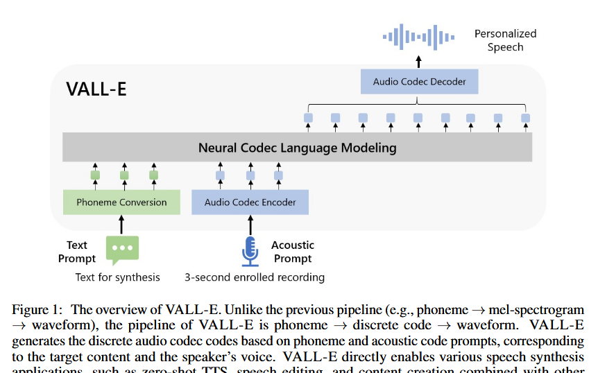
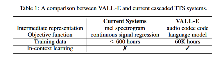
<p>VALL-E aimed to “regard TTS as a conditional language modeling task rather than continuous signal regression”. It did so by making use of latent spaces and by using a ton of data, scaling training data to 60,000 hours of speech. <br />
<img src="../assets/img/codec_post/valle_overview.png" alt="vall-e overview diagram" />
<a href="https://arxiv.org/pdf/2301.02111">Source</a></p>

<p><img src="../assets/img/codec_post/valle_comparison.png" alt="vall-e table diagram" />
<a href="https://arxiv.org/pdf/2301.02111">Source</a></p>

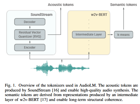
<p>AudioLM used a two-token approach: semantic tokens from <a href="https://arxiv.org/abs/2108.06209">w2v-BERT</a> for capturing “local dependencies (e.g., phonetics in speech, local melody in piano music) and global long-term structure (e.g., language syntax and semantic content in speech; harmony and rhythm in piano music)”; and acoustic tokens from an audio codec for capturing audio waveform structure and details.<br />
<img src="../assets/img/codec_post/audiolm_tokenizer.png" alt="AudioLM tokenizer diagram" />
	<a href="https://arxiv.org/pdf/2209.03143">Source</a></p>

<p>Because codecs and the intermediate representations they produce play such an integral role in this language modeling process, let’s take a closer look at the codecs used by these two models and examine in detail what the conversion process and results look like in practice.</p>

<h2 id="audio-tokens-and-codecs">Audio Tokens and Codecs</h2>

<p>In order to carry out this language modeling, the audio ML models used latent spaces in the form of <a href="https://en.wikipedia.org/wiki/Codec">codecs</a>, algorithms that encode data streams, in this instance the data streams being either the text of the spoken words or the audio itself in the form of a wave file. VALL-E used an algorithm called <a href="https://arxiv.org/pdf/2210.13438">EnCodec</a>, and AudioLM used one called <a href="https://arxiv.org/pdf/2107.03312">SoundStream</a>.</p>

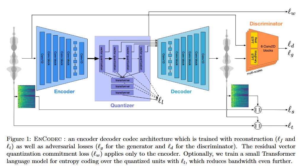
<p>EnCodec has three main components: an encoder network, a quantization layer, and a decoder.<br />
The whole system is trained end-to-end and minimizes a reconstruction loss over both the time and frequency domain. This diagram from the EnCodec paper displays the entire pipeline from end to end, showcasing the three components:<br />
<img src="../assets/img/codec_post/encodec_diagram.png" alt="Encodec diagram" /><br />
<a href="https://arxiv.org/pdf/2210.13438">Source</a></p>

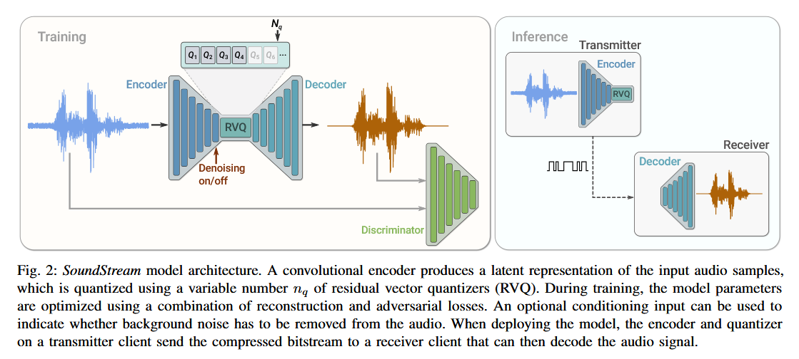
<p>SoundStream relies on a model architecture made up of a fully convolutional encoder/decoder network and a residual vector quantizer (RVQ). It also includes adversarial and reconstruction losses to allow the generation of high-quality audio content from quantized embeddings. The encoder receives as input a waveform and produces a sequence of embeddings at a lower sampling rate, which are quantized by the RVQ. The decoder can then reconstruct an approximation of the original waveform. <br />
The diagram below from the SoundStream paper gives an overview of the full system:<br />
<img src="../assets/img/codec_post/soundstream_diagram.png" alt="SoundStream diagram" /><br />
<a href="https://arxiv.org/pdf/2107.03312">Source</a></p>

<p>The paper also includes a breakdown of the steps of the model:<br />
<img src="../assets/img/codec_post/soundstream_steps.png" alt="SoundStream Steps" /><br />
	<a href="https://arxiv.org/pdf/2107.03312">Source</a></p>

<p><strong>Code example</strong><br />
To really drive home what an audio codec is doing, let’s <a href="https://github.com/facebookresearch/encodec">walk through</a> what it looks like to encode some audio in python using EnCodec.</p>

<p>First, we’ll load the EnCodec libraries and a sample audio file</p>

<div class="language-plaintext highlighter-rouge"><div class="highlight"><pre class="highlight"><code>from datasets import load_dataset, Audio  
from transformers import EncodecModel, AutoProcessor  
import torch

# dummy dataset, however you can swap this with an dataset on the 🤗 hub or bring your own  
librispeech_dummy = load_dataset("hf-internal-testing/librispeech_asr_dummy", "clean", split="validation")

# load the model + processor (for pre-processing the audio)  
model = EncodecModel.from_pretrained("facebook/encodec_24khz")  
processor = AutoProcessor.from_pretrained("facebook/encodec_24khz")

# cast the audio data to the correct sampling rate for the model  
librispeech_dummy = librispeech_dummy.cast_column("audio", Audio(sampling_rate=processor.sampling_rate))  
audio_sample = librispeech_dummy[0]["audio"]["array"]  
print(f"Input audio shape: {audio_sample.shape}")
</code></pre></div></div>

<p><code class="language-plaintext highlighter-rouge">Input audio shape: (140520,)</code></p>

<p>With that in place, we can preprocess the inputs and encode the audio sample</p>

<div class="language-plaintext highlighter-rouge"><div class="highlight"><pre class="highlight"><code>inputs = processor(raw_audio=audio_sample, sampling_rate=processor.sampling_rate, return_tensors="pt")

encoder_outputs = model.encode(inputs["input_values"], inputs["padding_mask"])
</code></pre></div></div>

<p>Examining the results, we see that the encoder has created a tensor in the latent space with a much smaller size than the input tensor. The actual values aren’t interpretible to us, as they represent a result in latent space.</p>

<div class="language-plaintext highlighter-rouge"><div class="highlight"><pre class="highlight"><code>detail_tensor = encoder_outputs['audio_codes']  
print(f"Tensor data type: {detail_tensor.dtype}")  
print(f"Tensor shape: {detail_tensor.shape}")  
print(f"Number of dimensions (rank): {detail_tensor.ndim}")  
print(f"Total number of elements: {detail_tensor.numel()}")
</code></pre></div></div>
<div class="language-plaintext highlighter-rouge"><div class="highlight"><pre class="highlight"><code>Tensor data type: torch.int64  
Tensor shape: torch.Size([1, 1, 2, 440])  
Number of dimensions (rank): 4  
Total number of elements: 880
</code></pre></div></div>
<p>To complete the process, we can call the decoder on the encoded value.</p>
<div class="language-plaintext highlighter-rouge"><div class="highlight"><pre class="highlight"><code>audio_values = model.decode(encoder_outputs.audio_codes, encoder_outputs.audio_scales, inputs["padding_mask"])[0]

print(f"Tensor data type: {audio_values.dtype}")  
print(f"Tensor shape: {audio_values.shape}")  
print(f"Number of dimensions (rank): {audio_values.ndim}")  
print(f"Total number of elements: {audio_values.numel()}")
</code></pre></div></div>
<div class="language-plaintext highlighter-rouge"><div class="highlight"><pre class="highlight"><code>Tensor data type: torch.float32  
Tensor shape: torch.Size([1, 1, 140520])  
Number of dimensions (rank): 3  
Total number of elements: 140520
</code></pre></div></div>
<p>When we play the resulting audio, we see it is close to the original, but slightly distorted, since the latent space encoding uses a statistical variational process, rather than being purely deterministic.</p>

<h1 id="moving-forward">Moving Forward</h1>

<p>With these advancements at the end of 2023/beginning of 2024, language modeling moved forward as the dominant method for TTS. Cutting edge research continues to use this paradigm; for instance, <a href="https://github.com/SparkAudio/Spark-TTS">SparkTTS</a> (2025) used a novel tokenizer called BiCodec, separating semantic tokens for meaning and global tokens for speaker content. <a href="https://microsoft.github.io/VibeVoice/">VibeVoice</a> (2025) used a specialized speech tokenizer as well.<br />
Experimentation with new ideas continues. Some researchers are investigating the move from discrete to <a href="https://arxiv.org/pdf/2507.09834">continuous</a> codes. Others are experimenting with a return to the simplification of the end-to-end pipeline system, <a href="https://github.com/SesameAILabs/csm">Sesame’s CSM</a> (2025) being a great example of that. Nevertheless, language modeling and audio codecs continue to play a key role in generative modeling of the audio space.</p>]]></content><author><name></name></author><summary type="html"><![CDATA[As I mentioned in my last post, one of the big developments in TTS architecture was the shift toward text to speech as a language modeling task with the use of audio tokens in the modeling process. In this post we’re going to dive into what that actually means and looks like in practice. We’ll start by giving a little bit of background looking briefly at the uses of latent spaces in earlier neural architectures. We’ll then see how latent spaces were applied to the audio domain, and we’ll take a closer look at the use of audio codes in this regard. So to begin, let’s explain what we mean by “latent spaces”.]]></summary></entry><entry><title type="html">TTS Architecture Trends</title><link href="/blog/tts_arch_trends" rel="alternate" type="text/html" title="TTS Architecture Trends" /><published>2026-02-11T00:00:00+00:00</published><updated>2026-02-11T00:00:00+00:00</updated><id>/blog/tts-arch-trends</id><content type="html" xml:base="/blog/tts_arch_trends"><![CDATA[<p>In my <a href="https://8t88.github.io/blog/tts_timeline.html">previous post</a>, I walked through major open-source models in the TTS audio generation space. The development of these models over time has followed different trends in terms of design decision tradeoffs as researchers aimed to improve the quality and performance of their models. In this post, I’m going to take a look at some of these key trends and the reasoning behind the design decisions. This post will be slightly more technical than the previous one. I’ll be focusing on the innovations that have been developed in the audio ML space, but I’ll be assuming you have some knowledge of how generative AI systems work (the basic ideas behind transformers, diffusion models, etc.)</p>

<p>As has taken place across all domains within machine learning, we’ve seen the natural progression of increased scaling in dataset size and model size. Beyond these increased magnitudes though, researchers and engineers have settled on several design decisions aimed at improving the speed and quality of audio generation. The two main topics I want to highlight are the general trends around the simplification of end-to-end pipeline system design, and the utilization of generative models including VAEs, Transformers, Adversarial Networks, and Diffusion models.</p>

<h1 id="pipeline-simplification">Pipeline Simplification</h1>

<p><img src="../assets/img/tts_arch_post/diagram.png" alt="arrows diagram" width="50%" /></p>

<h3 id="component-based-architecture">Component-based Architecture</h3>

<p>Prior to the shift in using Machine Learning for text to speech, traditional TTS systems performed the conversion by using multi-stage systems made from components such as text analysis, duration modeling, acoustic modeling, and a vocoder. These components would typically be implemented and tuned individually by audio engineers. While it worked well for its time, these systems were often brittle and difficult to expand upon because of their complexity.</p>

<h3 id="two-stage-systems">Two-Stage Systems</h3>

<p>A fundamental paradigm in the growth of ML was the increased emphasis on using the data to do the heavy lifting through neural nets, rather than individually tailored algorithms. To this end, <a href="https://arxiv.org/pdf/1609.03499">WaveNet</a> (2016) simplified the multi-component pipeline by replacing the vocoder and acoustic model components with a neural network structure; however, the neural nets were still conditioned on linguistic features such as the <a href="https://www.audiolabs-erlangen.de/resources/MIR/FMP/C3/C3S1_SpecLogFreq-Chromagram.html">logarithmic fundamental frequency</a> and phone durations. <br />
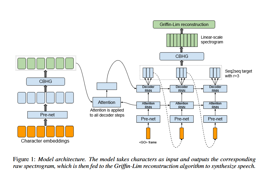
Following this, more models continued this trend toward a general two-stage system, where the text was converted to intermediate representations such as mel-spectrograms, and then those intermediate forms were converted into the final waveform. <a href="https://arxiv.org/pdf/1703.10135">Tacotron</a> (2017) did this by synthesizing speech from characters, while having an intermediate component that produced spectrograms to be passed to a reconstruction algorithm (Griffin-Lim). or a vocoder.</p>

<p><img src="../assets/img/tts_arch_post/tacotron_architecture.png" alt="tacotron arch diagram" />
<a href="https://arxiv.org/pdf/1703.10135">Tacotron Architecture</a></p>

<p>This was similarly the case with <a href="https://research.baidu.com/uploads/5ac03da1e126a.pdf">Deep Voice 3</a> (2017), which fed textual features (e.g. characters, phonemes, stresses)  into various vocoder parameters, such as mel-band spectrograms, linear-scale log magnitude spectrograms, fundamental frequency, spectral envelope, and aperiodicity.</p>

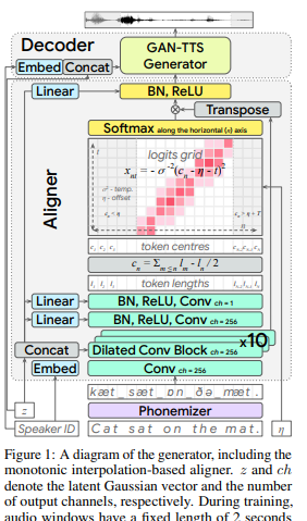
<p>This trend gradually continued up to the 2020s, when researchers really tried to lean more fully into getting rid of these component-based systems by replacing them with single stage end-to-end models. These systems would take in waveforms, pass them through transformer/diffusion architectures, then output the speech result. <br />
<a href="https://arxiv.org/abs/2006.03575">EATS</a> (2020) was a clear example of this; it operated directly on character or phoneme input sequences and produced raw speech audio output. It was composed of two high-level submodules: an aligner, which processed the raw input sequence and converted them into a latent feature space; and the decoder, which turned those features into 24 kHz audio waveforms. <br />
<img src="../assets/img/tts_arch_post/eats_architecture.png" alt="eats arch diagram" /></p>

<p><a href="https://arxiv.org/pdf/2006.03575">EATS architecture</a></p>

<p><a href="https://arxiv.org/pdf/2106.06103">VITS</a> (2021) tried to go even further by making a true single stage pipeline using VAEs guided by normalizing flows and an adversarial training process</p>

<h3 id="audio-tokens-and-language-modeling">Audio Tokens and Language Modeling</h3>

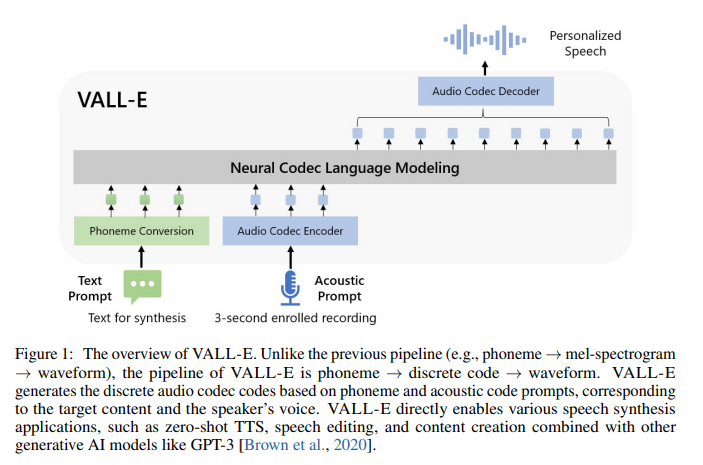
<p>After experimenting with this strategy for a couple of years, developers took a slight step back toward the component based approach by modeling discrete audio tokens then using those to generate the speech results. This coincided with the move toward adopting transformer architectures (more on that in the <a href="#model-technologies">next section</a>). Some early examples of these were <a href="https://research.google/blog/audiolm-a-language-modeling-approach-to-audio-generation/">AudioLM</a> (2022) and <a href="https://www.microsoft.com/en-us/research/project/vall-e-x/">VALL-E</a> (2023). VALL-E innovated by replacing intermediate acoustic representations of mel spectrograms with discrete <a href="https://en.wikipedia.org/wiki/Audio_codec">audio codec</a> codes.<br />
<img src="../assets/img/tts_arch_post/valle_architecture.png" alt="vall-e arch diagram" />
<a href="https://arxiv.org/pdf/2301.02111">VALL-E Architecture</a></p>

<p>As of Now, the audio token approach is still producing the top results, but many models in 2025 attempted to return to the single stage simplification seen earlier, particularly in single-transformer models like <a href="https://llasatts.github.io/llasatts/">Llasa</a> and end-to-end pipelines like <a href="https://github.com/SesameAILabs/csm">Sesame CSM</a></p>

<h1 id="model-technologies">Model Technologies</h1>

<p>Prior to the mid-2010s, TTS systems relied on classical signal processing and statistical modeling to speech waveforms. As the machine learning and then generative ai space took off, developers incorporated these new algorithms and models to generate more realistic speech results.</p>

<h3 id="cnns-and-rnns">CNNs and RNNs</h3>

<p>In the second half of the 2010s, the leading edge of ML development took the form of Deep Learning composed of <a href="https://en.wikipedia.org/wiki/Convolutional_neural_network">CNNs</a> and <a href="https://en.wikipedia.org/wiki/Recurrent_neural_network">RNNs</a>. Consequently, systems like WaveNet, Tacotron, and Deep Voice all incorporated these architectures into their pipelines.</p>

<h3 id="encodersdecoders-transformers-and-adversarial-nets">Encoders/Decoders, Transformers, and Adversarial Nets</h3>

<p>By the end of the 2010s and going into the 20s, developers started to incorporate the leading <a href="https://deepgenerativemodels.github.io/notes/">generative models</a> into their systems. <br />
Adversarial training was added as a component to the training of several TTS systems, EATS being an early example, followed by VITS. <br />
Additionally, new systems moved from using CNNs and RNNs to making use of encoder-decoder structures and Transformers. DeepVoice 3 in 2018 was an early example of this, it used a convolutional encoder-decoder and was attention-based. Additionally, VITS used <a href="https://deepgenerativemodels.github.io/notes/vae/">VAEs</a> in tandem with the adversarial components mentioned above. <br />
However, the use of Transformers in TTS architecture really started getting more widely adapted around 2022, when the <a href="#audio-tokens-and-language-modeling">trend moved toward TTS as a language modeling task</a> rather than a direct conversion mechanism. This is because the process of converting data to tokens lent itself naturally to the Transformer’s structure.</p>

<h3 id="diffusion-models">Diffusion Models</h3>

<p>On top of this, many of the models added a diffusion component on top of the transformer encoder/decoder mechanisms to generate the final audio output and produce a more natural sound. <a href="https://github.com/neonbjb/tortoise-tts">TorToise</a> (2023) and <a href="https://arxiv.org/abs/2306.07691">StyleTTS2</a> (2023) were notable in this regard. This fusion of transformers and diffusion models has continued to the present, with models like <a href="https://index-tts.github.io/index-tts2.github.io/">IndexTTS2</a> (2025) using this approach.</p>

<h1 id="bonus-autoregressive-modeling">Bonus: Autoregressive modeling</h1>

<h3 id="pros-and-cons">Pros and Cons</h3>

<p><a href="https://deepgenerativemodels.github.io/notes/autoregressive/">Autoregressive (AR) models</a> are models where outputs are modeled based on previous values. <br />
Unlike the other trends we’ve highlighted that have a general direction of development, the use of Autoregressive modeling in TTS systems has actually gone back and forth over the years, as  developers have weighed the tradeoffs between the two.<br />
AR architectures give high-quality outputs and generally improve results, but they can be slow. They are also sequential and thus inherently unparallelizable Consequently, Non-Autoregressive (NAR) methods may be chosen when speed or performance is of high value, depending on the use case. Additionally, NAR methods can work better with some of the other trends that architectures have taken; in particular the exponential growth of datasets and parameter counts can be enabled by the use of NAR methods, to get the system to actually finish training. However, NAR models have challenges of their own, such as difficulty in maintaining alignment between input text and synthesized speech.</p>

<h3 id="back-and-forth">Back and Forth</h3>

<p>Starting with WaveNet and continuing on in others such as Tacotron and Deep Voice, an  autoregressive architecture was used as it produced positive results. <br />
<a href="https://arxiv.org/abs/1811.00002">WaveGlow</a> (2018) was an early attempt at moving away from using an autoregressive system, followed by EATS and VITS. This didn’t take hold too strongly though, and many other systems continued to use AR methods. For instance, VALL-E used an autoregressive model for coarse tokens and a Non-Autoregressive model for fine residual tokens. <a href="https://www.microsoft.com/en-us/research/project/e2-tts/">E2-TTS</a> (2024) on the other hand, was fully Non-Autoregressive.<br />
In the latest stage of events, AR has been incorporated once again, with Llasa, <a href="https://github.com/SparkAudio/Spark-TTS">Spark-TTS</a> (2025), and <a href="https://microsoft.github.io/VibeVoice/">VibeVoice</a> (2025) all incorporating autoregressive components into their system.</p>

<h1 id="final-thoughts">Final Thoughts</h1>

<p>Here in 2026 there is still much R&amp;D being conducted in the audio generation space. Researchers continue to experiment with architectures to achieve new levels of realism in speech generation. Some other developments we’ve seen recently are:</p>

<ul>
  <li>Distillation into smaller models (often with Llama3 as backbone). This is in contrast to the increased model sizes mentioned above, and is of interest because it shows high quality outputs can be produced from much smaller inference</li>
  <li>Compute resources strategies, in the same vein as inference-time focus with reasoning models. Llasa demonstrates that scaling training-time and inference-time compute can significantly refine prosody and accuracy</li>
  <li>Multilanguage; largely a component of the increased data size as well as the language modeling paradigm shift</li>
</ul>

<p>Stay tuned for future posts, where we’ll take a closer look at some of the design components we’ve discussed, and eventually take a deeper dive into the models themselves.</p>]]></content><author><name></name></author><summary type="html"><![CDATA[In my previous post, I walked through major open-source models in the TTS audio generation space. The development of these models over time has followed different trends in terms of design decision tradeoffs as researchers aimed to improve the quality and performance of their models. In this post, I’m going to take a look at some of these key trends and the reasoning behind the design decisions. This post will be slightly more technical than the previous one. I’ll be focusing on the innovations that have been developed in the audio ML space, but I’ll be assuming you have some knowledge of how generative AI systems work (the basic ideas behind transformers, diffusion models, etc.)]]></summary></entry><entry><title type="html">A Timeline of TTS models</title><link href="/blog/tts_timeline" rel="alternate" type="text/html" title="A Timeline of TTS models" /><published>2026-01-05T00:00:00+00:00</published><updated>2026-01-05T00:00:00+00:00</updated><id>/blog/tts-timeline</id><content type="html" xml:base="/blog/tts_timeline"><![CDATA[<h3 id="a-decade-of-innovation">A Decade of Innovation</h3>

<p>Audio data has always captured my interest the most out of the various machine learning modalities. This is largely because of its seeming esoteric nature, particularly when it comes to speech vocalizations. If you were to look at a waveform plot or a spectrogram, it isn’t readily apparent how these data outputs map to words and phrases. With the explosive growth of generative machine learning in the past decade, I’ve tried to keep informed about the development of audio modeling, especially Text-to-Speech (TTS) systems.</p>

<p>The way I see it, audio has been the overlooked third child in the family of modalities, with its older siblings of text and image taking much of the spotlight. Technical challenges may have contributed to this: the data rate for audio is significantly higher than text, and there is a one-to-many relationship between text and audio, meaning that the same sentence can be rendered by different speakers with different speaking styles, emotional content, and recording conditions. Or maybe the lack of focus has just been because of people’s tastes. Whatever the reason, the capabilities of machine learning to generate audio recordings is only now reaching the level of astonishing realism we’ve gotten from text and image generation.</p>

<p>This post walks through the major Text-to-Speech models focused on or contributing to this development of audio generation, starting back in 2016. There are plenty of forks and project-spinoffs out there, but these are openly published (<a href="https://arstechnica.com/information-technology/2024/08/debate-over-open-source-ai-term-brings-new-push-to-formalize-definition/">loosely speaking</a>) models I’ve found to have gotten significant attention from their innovations or the resources devoted to them, and have led the way to our current state of the art. In later posts, I plan to compare/contrast the methodology and architectures these models use, and then deep dive into some specific models that I think are particularly interesting.</p>

<p>So let’s go back in time, starting in a year before we realized that Attention was all we needed…</p>

<h2 id="2016">2016</h2>

<h3 id="wavenet"><a href="https://arxiv.org/pdf/1609.03499">WaveNet</a></h3>

<p>Starting things off in the pre-transformer days, Google’s WaveNet was the first major model to successfully use the raw waveform of the audio signal for input data, as opposed to feature engineering <a href="https://haythamfayek.com/2016/04/21/speech-processing-for-machine-learning.html">acoustic features</a>. It uses an autoregressive architecture.<br />
This model was a significant advancement over the then state-of-the-art methods built with parametric and concatenative systems, and was able to generate English and Mandarin speech.</p>

<h2 id="2017">2017</h2>

<h3 id="deep-voice"><a href="https://research.baidu.com/uploads/5ac03da1e126a.pdf">Deep Voice</a></h3>

<p>Baidu iterated upon Deep Voice with some modifications and optimizations, first releasing Deep Voice 2 in March 2017. This was followed by a complete architectural redesign resulting in <a href="https://arxiv.org/abs/1710.07654">Deep Voice 3</a>, released October 2017. The redesign transformed the system from a combination of multiple neural networks into a single encoder-decoder design.</p>

<h3 id="tacotron"><a href="https://arxiv.org/pdf/1703.10135">Tacotron</a></h3>

<p>Another research development from Google, this system aimed to generate speech directly from text characters, rather than using the more prevalent at the time approach of multiple pipeline components including a linguistic feature extractor, vocoder, etc. The model took in &lt;text,audio&gt; pairs, transformed them into spectrograms, and trained on that data to produce waveforms. <br />
This sequence-to-sequence model uses an encoder-decoder architecture and an attention mechanism, potentially making it the first major text-to-speech transformer model.</p>

<h2 id="2018">2018</h2>

<h3 id="waveglow"><a href="https://arxiv.org/abs/1811.00002">WaveGlow</a></h3>

<p>Submitted October 2018, this flow-based network model was built by Nvidia and used ideas from WaveNet and OpenAI’s <a href="https://openai.com/index/glow/">Glow</a>. Similar models include Glow-TTS and Flow-TTS. The system uses a diffusion model, taking mel-spectrograms as inputs, and is implemented with a single network for greater simplicity. <br />
One of the key design decisions of WaveGlow was to move away from an autoregressive system. While useful, autoregressive TTS systems are inherently sequential so have the downside of not being very parallelizable.</p>

<h2 id="2019">2019</h2>

<h3 id="wav2vec"><a href="https://huggingface.co/facebook/wav2vec2-large-960h-lv60-self">wav2vec</a></h3>

<p><a href="https://ai.meta.com/blog/wav2vec-20-learning-the-structure-of-speech-from-raw-audio/">Released</a> by Meta in April 2019 and followed by wav2Vec 2.0 in 2020, this system uses raw, unlabeled audio to train automatic speech recognition models. It was trained by predicting speech units for masked parts of the audio, learning basic units that are 25ms long to enable learning of high-level contextualized representations</p>

<h2 id="2020">2020</h2>

<h3 id="eats-end-to-end-adversarial-text-to-speech"><a href="https://arxiv.org/abs/2006.03575">EATS (End-to-End Adversarial Text-to-Speech)</a></h3>

<p>Released by DeepMind in June 2020, this system uses phonemes in an “end-to-end” manner, rather than having multiple processing stages (such as text normalisation, aligned linguistic featurization, mel-spectrogram synthesis, and raw audio waveform synthesis) The drawback of these multi-component systems is that they need extra training and tuning for each step of the pipeline, however the results appeared very promising.</p>

<h2 id="2021">2021</h2>

<h3 id="vits"><a href="https://huggingface.co/docs/transformers/en/model_doc/vits">VITS</a></h3>

<p>Released June 2021, this model also tried to <a href="https://github.com/jaywalnut310/vits/">implement</a> a parallel end-to-end autoencoder system that matched the quality of two-stage systems. It used variational inference augmented with normalizing flows and an adversarial training process.<br />
This was followed by VITS2 in 2023, which <a href="https://github.com/daniilrobnikov/vits2">implemented</a> some structure and training improvements</p>

<h3 id="huberthidden-unit-bert"><a href="https://arxiv.org/abs/2106.07447">HuBERT(Hidden-Unit BERT)</a></h3>

<p>While not technically a TTS system, this model is worth highlighting because of its use in other systems.<br />
Basically, this was Meta’s development of <a href="https://research.google/blog/open-sourcing-bert-state-of-the-art-pre-training-for-natural-language-processing/">BERT</a> for audio. Like, BERT, HuBERT, gets used in other audio models and processing tasks, such as <a href="#heading=h.u0hhx0p1vuog">RVC</a><br />
At a high level, HuBERT takes in a float array corresponding to the raw waveform of the speech signal and passes it to a wav2vec2.0 model to encode it. The final output is a feature sequence, and on that output the model uses a clustering step to create “hidden units”.<br />
Read <a href="https://jonathanbgn.com/2021/10/30/hubert-visually-explained.html">here</a> for a great in-depth examination of this system.</p>

<h2 id="2022">2022</h2>

<p>2022 was the year that gen AI really hit the public consciousness, with the releases of Dall-E 2 and ChatGPT. While primary focus was on textual and visual results, this year still saw some very interesting experimentation and development in the audio space.</p>

<h3 id="styletts"><a href="https://styletts.github.io/">StyleTTS</a></h3>

<p>The <a href="https://arxiv.org/abs/2205.15439">StyleTTS paper</a> was initially submitted May 2022 and was followed-up by the <a href="https://arxiv.org/abs/2306.07691">StyleTTS2</a> paper in June 2023 along with a code <a href="https://styletts.github.io/">implementation</a>. The goal was to develop a better parallel TTS system that improves on the deficiencies in other systems around aligning monotonic speech segments. The system uses an encoder-decoder architecture to generate a mel-spectrogram from text while incorporating parallel encoder blocks to be able to incorporate information around “style”, e.g. prosodic patterns and emotional tone. It also introduced an innovation called a Transferable Monotonic Aligner (TMA) to set the duration generation. <br />
This system has given rise to some interesting <a href="https://github.com/NeuralVox/StyleTTS2">forks</a>, <a href="https://github.com/IIEleven11/StyleTTS2FineTune?tab=readme-ov-file">fine-tunes</a>, and eventual <a href="#kokoro">offshoots</a>.</p>

<h3 id="audiolm"><a href="https://research.google/blog/audiolm-a-language-modeling-approach-to-audio-generation/">AudioLM</a></h3>

<p>Released by Google in October 2022. This model aims to generate realistic speech (and piano music) by listening to audio only.<br />
The system extracts semantic tokens using <a href="https://arxiv.org/abs/2108.06209">w2v-BERT</a>, as well as acoustic tokens produced by <a href="https://ai.googleblog.com/2021/08/soundstream-end-to-end-neural-audio.html">a SoundStream neural codec</a>, and passes these tokens through multiple transformer models. To get the final result, the SoundStream decoder converts the encoded tokens into a waveform. This was done for research purposes only, so although the paper described the details of the architecture, the weights and code were not released.</p>

<h2 id="2023">2023</h2>

<p>With the sky opened and the belief in GenAI soaring, 2023 was a year when the amount of new TTS models really started to take off, with some very impressive and innovative systems appearing that still see a little bit of use today.</p>

<h3 id="piper"><a href="https://piper.ttstool.com/">Piper</a></h3>

<p>This is a TTS engine and a set of voice packs built by the Piper Project, from the <a href="https://www.openhomefoundation.org/">Open Home Foundation</a>. It is a small model that uses the <a href="#vits">VITS</a> architecture. The initial release came in January 2023, and it continues to be open-sourced and developed.</p>

<h3 id="parlertts"><a href="https://github.com/huggingface/parler-tts/tree/main">ParlerTTS</a></h3>

<p>A reproduction of the work described in the paper <a href="https://www.text-description-to-speech.com/">Natural language guidance of high-fidelity text-to-speech with synthetic annotations</a>, Parler-TTS is an auto-regressive transformer-based model, with the aim of being lightweight and producing natural-sounding speech.</p>

<h3 id="vall-e"><a href="https://www.microsoft.com/en-us/research/project/vall-e-x/">VALL-E</a></h3>

<p>The next offering from Microsoft would appear in 2023 as <a href="https://arxiv.org/pdf/2301.02111">VALL-E</a>. Unlike other text-to-speech methods that typically synthesize speech by manipulating waveforms, VALL-E generates discrete audio codec codes from text and acoustic prompts. It basically analyzes how a person sounds, breaks that information into discrete components (called “tokens”) using EnCodec, and uses training data to match what it “knows” about how that voice would sound if it spoke other phrases outside of the three-second sample.<br />
It was a pioneer in trying out language modeling for zero-shot TTS (TTS not trained for one specific speaker).</p>

<h3 id="bark"><a href="https://huggingface.co/suno/bark">Bark</a></h3>

<p>This transformer based model was open-sourced by <a href="http://suno.ai">suno.ai</a> in April 2023. The system consists of three components that form a pipeline: text-to-semantic tokens, semantic-to-coarse tokens, and coarse-to-fine tokens.<br />
This model was aimed toward producing more natural-sounding speech, as results generated contain non-verbal aspects such as laughing, as well as verbal tics of “umm”, “uh”, etc.<br />
While no longer maintained, this model can still be useful as a reference point or for research purposes.</p>

<h3 id="tortoise"><a href="https://github.com/neonbjb/tortoise-tts">TorToiSe</a></h3>

<p>This model is where I think we begin to see the ice breaking around truly impressive speech generation. Rumored by many to be the basis of ElevenLabs’ technological suite, the TorToiSe model, named thus to underscore how <em>slow</em> it is, uses both an autoregressive encoder-decoder as well as a diffusion component to enhance its ability to model in the continuous domain and focus on reproducing human voices realistically. <br />
TorToiSe provides the autoregressive generator and DDPM with a “speech conditioning input”, a unique design choice intended to allow the model to infer vocal characteristics like tone and prosody. In addition to the <a href="https://arxiv.org/pdf/2305.07243">paper</a>, you can read more about the design details <a href="https://nonint.com/2022/04/25/tortoise-architectural-design-doc/">here</a>.</p>

<h3 id="audiopalm"><a href="https://google-research.github.io/seanet/audiopalm/examples/">AudioPaLM</a></h3>

<p>Released June 2023, this system combines two Google language models, PaLM-2 and AudioLM, into a multimodal architecture. It inherits the speaker identification and intonation copying capabilities from AudioLM, and the linguistic abilities of LLM from PaLM-2.</p>

<h3 id="seamlessm4t"><a href="https://about.fb.com/news/2023/08/seamlessm4t-ai-translation-model/">SeamlessM4T</a></h3>

<p>Released by Meta in August 2023, this model performs text to speech as well as speech-to-speech and speech-to-text.<br />
An all-in-one model, it uses self-supervised speech representations with w2v-BERT 2.0, then uses the aligned the speech translations for training.</p>

<h2 id="2024">2024</h2>

<p>Riding high on the momentum of 2023, this year saw even greater expansion and improvements. While companies such as OpenAI and Anthropic deployed closed systems with multimodal capabilities that could produce very impressive audio, open-source developments and modifications continued to emerge and push the space forward.</p>

<h3 id="gpt-sovits-v2"><a href="https://rentry.co/GPT-SoVITS-guide#/">GPT-SoVITS-v2</a></h3>

<p>Connected to the team involved with the <a href="https://github.com/RVC-Project/Retrieval-based-Voice-Conversion-WebUI">RVC voice changer</a> and released in February 2024, this model generates acoustic tokens with a seq2seq model then converts those tokens into waveforms. Deep dives can be found <a href="https://blog.openvino.ai/blog-posts/openvino-enable-digital-human-tts-gpt-sovits">here</a> and <a href="https://medium.com/axinc-ai/gpt-sovits-a-zero-shot-speech-synthesis-model-with-customizable-fine-tuning-e4c72cd75d87">here</a>.</p>

<h3 id="metavoice"><a href="https://github.com/metavoiceio/metavoice-src">Metavoice</a></h3>

<p>Released in February 2024, this model predicts EnCodec tokens from text, and uses speaker information to condition the input at the token embedding layer. It then uses multi-band diffusion to generate waveforms from the EnCodec tokens, and concludes by passing the result through a DeepFilterNet to help clear up artifacts. The system also supports KV-caching via Flash Decoding and batching.</p>

<h3 id="melotts"><a href="https://huggingface.co/myshell-ai/MeloTTS-English">MeloTTS</a></h3>

<p>A multi-lingual text-to-speech library by MIT and <a href="http://MyShell.ai">MyShell.ai</a>, this system was first released in February 2024. <br />
The implementation is based on <a href="https://github.com/coqui-ai/TTS">TTS</a>, <a href="https://github.com/jaywalnut310/vits">VITS</a>, <a href="https://github.com/daniilrobnikov/vits2">VITS2</a> and <a href="https://github.com/fishaudio/Bert-VITS2">Bert-VITS2</a>. The open-source codebase also <a href="https://github.com/myshell-ai/MeloTTS/blob/main/docs/training.md">provides</a> some boilerplate to let you train and fine-tune the model on your own data.</p>

<h3 id="e2-tts"><a href="https://www.microsoft.com/en-us/research/project/e2-tts/">E2-TTS</a></h3>

<p>Another model from Microsoft Research, this non-autoregressive system was released June 2024. It uses only two modules, the flow-matching Transformer and the vocoder, eschewing additional components such as a duration model or grapheme-to-phoneme converter. It also does not use monotonic alignment or cross-attention.<br />
Despite detailing the architecture in the paper, this system was not open-sourced, but it was reverse-engineered by the <a href="#f5-tts">F5-TTS</a> team as well as <a href="https://github.com/lucidrains/e2-tts-pytorch">some others</a>.</p>

<h3 id="xtts"><a href="https://arxiv.org/abs/2406.04904">XTTS</a></h3>

<p>Coming out in June 2024, this system built upon the TorToiSe model, with some modifications.<br />
It aimed to expand language capabilities much wider to cover 16 languages, as well as provide cross-language zero-shot TTS without needing a parallel training dataset.<br />
The system takes in a  mel-spectrogram as input, and it makes use of a VQ-VAE, the GPT-2 encoder, as well as a HifiGAN model to compute the final audio signal<br />
A deeper dive into the system can be found <a href="https://erogol.com/2023/11/11/xtts-v2-release-and-notes">here</a>.</p>

<h3 id="f5-tts"><a href="https://swivid.github.io/F5-TTS/">F5-TTS</a></h3>

<p>Released in October 2024, F5 is a non-autoregressive text-to-speech system based on flow matching with a Diffusion Transformer. It follows in the flow-matching footsteps of <a href="#e2-tts">E2-TTS</a> but tries to make the design easier to follow and improves training time and performance. F5 also adds some additional innovations such as an inference-time Sway Sampling strategy.</p>

<h2 id="2025">2025</h2>

<p>While the models of 2024 produced impressive results, 2025 may have been the year when the uncanny valley was crossed. The models being released could not only produce natural-sounding audio, but they could also convincingly transfer outputs across accents or even languages.<br />
This year also saw more companies popping up as competitors to ElevenLabs, either centered on audio generation or incorporating it into multimodal AI agents and general world models. Furthermore, models such as <a href="#kokoro">Kokoro</a> and <a href="#spark-tts">Spark-TTS</a> would be released that could produce fast and impressive results from extremely small models.</p>

<h3 id="kokoro"><a href="https://huggingface.co/hexgrad/Kokoro-82M">Kokoro</a></h3>

<p>This model is built with StyleTTS2 as a backbone, though it’s not properly a distillation because it also removes parts of the original base model such as several utility models used during training in order to make it smaller. Although only the inference code and weights were released, this system got a lot of attention for its very small size while still producing impressive results. <br />
In addition to the trimming described above, another reason for its small model parameter count is that it doesn’t use a dynamic style diffusion method and instead uses ‘voicepacks’ for voice style transfer. Additionally, Kokoro outsources tokenization and phonemization, so that the only thing the model sees is phonemes and punctuation, further reducing the size.</p>

<h3 id="llasa"><a href="https://llasatts.github.io/llasatts/">Llasa</a></h3>

<p>Released around the beginning of February, the team behind Llasa had two main goals:</p>

<ul>
  <li>Explore the scaling of train-time and inference-time compute for speech synthesis</li>
  <li>Provide a simplified framework with single-layer vector quantizer (VQ) codec and a single Transformer architecture</li>
</ul>

<p>The researchers argued that a simplified architecture, like the transformer for text LLMs, allows for faster scientific exploration and progress. The scaling of train-time compute (e.g., increasing model size or training data) also consistently improves the naturalness of and expressiveness of the results.<br />
The system first uses Llama 3B (could also use 1B or 8B) to predict “speech tokens from the <a href="https://huggingface.co/HKUSTAudio/xcodec2">XCodec2</a> codebook, and then decodes these tokens into audio.</p>

<h3 id="zonos"><a href="https://huggingface.co/Zyphra">Zonos</a></h3>

<p>The Zonos models were first <a href="https://www.zyphra.com/post/beta-release-of-zonos-v0-1">released</a> in February 2025 by Zyphra, a company whose mission is “to build human-aligned AI that helps individuals and organizations reach their fullest potential”.<br />
The company released two models, the <a href="https://huggingface.co/Zyphra/Zonos-v0.1-transformer">1.6B transformer</a> and <a href="https://huggingface.co/Zyphra/Zonos-v0.1-hybrid">1.6B hybrid</a> (SSM model, first open-source of its kind for TTS) under an Apache 2.0 license, with the goal of highly expressive and natural-sounding audio that attempts to capture emotional variation. <br />
The transformer model uses an autoregressive pipeline, and makes use of audio tokens from <a href="https://github.com/descriptinc/descript-audio-codec">DAC vocoder</a>. It also takes a speaker embedding as an input for voice cloning capabilities, as well as other inputs such as speaking rate, pitch, sample rate, audio quality, and speaker emotions, producing speech outputs that are 44KHz.<br />
While it produces high quality outputs, some weaknesses include: audio artifacts at the beginning and end of generations; mistakes in text alignment (skipping words, repeated words, etc); and high quality but slower and more expensive inference. The model attempts to mitigate these by implementing some techniques such as: a delay codebook pattern from <a href="https://huggingface.co/parler-tts">Parler TTS</a>, multi-token prediction, and embedding merging.</p>

<h3 id="sesame-csm"><a href="https://github.com/SesameAILabs/csm">Sesame CSM</a></h3>

<p>With Sesame we see another company moving into the audio-generation field aimed at achieving as natural an experience as possible, as if you were actually speaking to someone in the real world. Their goal is to achieve “voice presence”, and the key component aims are: emotional awareness, conversational dynamics, contextual awareness, and consistent personality.<br />
The Conversational Speech Model (CSM) was released February 2025. The CSM has three sizes: Tiny (1B backbone, 100M decoder), Small (3B backbone, 250M decoder), and Medium (8B backbone, 300M decoder).<br />
Sesame’s CSM is a single-stage model, as opposed to a model using a two-step process of generating semantic tokens followed by acoustic tokens (commonly with <a href="https://arxiv.org/abs/2107.03312">RVQ</a>). The downside of a two-step is that it is difficult to ensure the semantic tokens fully capture the prosody during training. Also, RVQ can have a high latency.<br />
The model incorporates two autoregressive transformers, both variants of the Llama architecture. This requires a high level of memory, so the system uses compute amortization to help alleviate the memory footprint.<br />
More detailed info can be found in the <a href="https://www.sesame.com/research/crossing_the_uncanny_valley_of_voice">release announcement</a>.</p>

<h3 id="indextts"><a href="https://index-tts.github.io/">IndexTTS</a></h3>

<p>Released in Feb 2025 by the Index SpeechTeam, this system was based on XTTS and aimed at improvements over other popular TTS systems by utilizing a simpler training process, more controllable usage, and faster inference speed. This was followed by <a href="https://index-tts.github.io/index-tts2.github.io/">IndexTTS2</a> later in the year, which introduced some innovative techniques addressing the issue of audio-visual synchronization, with a primary use case of video dubbing. While still using an autoregressive model, this system makes use of methods for speech duration control and gives independent control over timbre and emotion.</p>

<h3 id="spark-tts"><a href="https://github.com/SparkAudio/Spark-TTS">Spark-TTS</a></h3>

<p>Built using Qwen 2.5, this system is similar to <a href="#llasa">Llasa</a> but much smaller and with great results. Instead of relying on separate models to generate acoustic features, it directly reconstructs audio from the code predicted by the LLM.</p>

<h3 id="orpheus"><a href="https://huggingface.co/collections/canopylabs/orpheus-tts-67d9ea3f6c05a941c06ad9d2">Orpheus</a></h3>

<p><a href="https://canopylabs.ai/model-releases">Released</a> in March by Canopy Labs, these models come in four different sizes, ranging from 3 billion parameters to 150 million parameters. The architecture uses Llama-3b as the backbone but utilizes two nonstandard design decisions: 7 tokens per sample frame decoded as a single flattened sequence, and using a non-streaming (CNN-based) tokenizer. The <a href="https://huggingface.co/collections/canopylabs/orpheus-tts">weights</a> and <a href="https://github.com/canopyai/Orpheus-TTS">code</a> are all open-sourced under an Apache-2.0 license.</p>

<h3 id="outetts"><a href="https://github.com/edwko/OuteTTS">OuteTTS</a></h3>

<p>Though some initial versions of OuteTTS started to get released at the end of 2024, this system went through a couple of iterations until OuteAI <a href="https://outeai.com/blog/outeai-1.0-update">released</a> the first major version of their toolsuite utilizing these models in June 2025. As of the end of 2025, the most advanced model is the <a href="https://huggingface.co/OuteAI/Llama-OuteTTS-1.0-1B">Llama-OuteTTS-1.0-1B</a>, While details about any innovations are scarce, this gives yet another example of an organization attempting to build a software product around audio generation while open-sourcing their TTS models.</p>

<h3 id="vibevoice"><a href="https://microsoft.github.io/VibeVoice/">VibeVoice</a></h3>

<p>An open-source development from Microsoft, this model was released to the public in August and comes in three sizes: 0.5B, 1.5B, and Large. It supports streaming text input as well as long-form generation. It uses an “interleaved, windowed design”, where the text chunks are encoded in parallel as they come in while the audio is generated from a diffuse-based model.</p>

<h3 id="maya1"><a href="https://huggingface.co/maya-research/maya1">Maya1</a></h3>

<p>For the final entry in our timeline, another model built with the Llama-3B backbone was released in October from Maya Research. This model uses a 3B-parameter decoder-only transformer (Llama-style) to predict SNAC neural codec tokens instead of raw waveforms. Besides the small size, the emphasis here is on creating emotionally expressive outputs of any type of voice described. The result is an impressive showing from a small research group and is one to keep an eye on in the future.</p>

<h2 id="closing-thoughts">Closing Thoughts</h2>

<p>With this, we’ve made our way to the beginning of 2026. I’m sure there are many models that I’ve missed, but I tried to capture important or particularly interesting ones that have shaped the conversation over the past decade.<br />
I hope you’ve enjoyed this high-level walkthrough of TTS history. Stay tuned for an upcoming post, where I’ll take a stab at digging into some of the major design decisions and tradeoffs that have shaped this history. Happy New Year everyone!</p>]]></content><author><name></name></author><summary type="html"><![CDATA[A Decade of Innovation]]></summary></entry></feed>